The R package StrucDiv contains methods to quantify scale-specific and multi-scale spatial structural diversity. Spatial structural diversity refers to the spatial, i.e. horizontal, configuration of landscape elements. Hereafter, ‘spatial structural diversity’ will be used synonymous to ‘structural diversity.’ The StrucDiv package provides methods to quantify structural diversity in continuous raster data. With these methods, structural diversity features can be detected. Structural diversity features have also been called latent landscape features. Typical structural diversity features include patches and linear landscape features and reveal transition zones between spatial regimes. Structural diversity can also be quantified in categorical raster data, required method specifications are described in Schuh, Santos, de Jong, et al. (2022). Structure is quantified by considering the spatial arrangement of pixel values as pairs, based on Haralick, Shanmugam, and Dinstein (1973). Structural diversity can be quantified on different spatial scales, whereby pixel resolution is an input to these methods, and different extents can be implemented. Scale-specific structural diversity can be quantified, either of the domain, or of smaller areas therein. The latter is done with a moving window approach. Multi-scale structural diversity is quantified by combining information from different scales (i.e. extents), as further described below. The methods are described in detail in Schuh, Santos, de Jong, et al. (2022) and in Schuh, Santos, Schaepman, et al. (2022), and the R package is described in Schuh and Furrer (2022). The R package contains three main functions:
strucDiv():
Scale-specific structural diversity quantificationThe strucDiv() function quantifies structural diversity
on a particular scale, which is defined by the size of the moving
window. Within the area captured by the moving window, pixel values are
considered as pairs at user defined distance and angle. A
direction-invariant version is available. The frequencies of value pair
occurrences are normalized by the total number of pixel pairs, which
returns the gray level co-occurrence matrix (GLCM). The GLCM contains
the empirical probabilities pi, j
that pixel values vi and vj
occur as a pair at the specified distance and angle(s), in the area
captured by the moving window. Structural diversity is based on
empirical probabilities of value co-occurrence. The output map is called
a ‘(spatial) structural diversity map’ and it is returned as a raster
layer. The output map represents structural diversity quantified on a
specific scale. This method is described in detail in Schuh, Santos, de
Jong, et al. (2022).
strucDivNest():
Multi-scale structural diversity quantificationThe strucDivNest() function allows to combine
information from different scales with an empirical Bayesian approach
and a Beta-Binomial model. Two scales are nested inside each other - a
larger, outer scale and a smaller, inner scale. Three different nesting
schemes are available, whereby the inner scale is always a moving
window. The outer scale can either be another mowing window, a block, or
the domain (i.e. the input raster). The outer scale is used as prior
information, and the inner scale serves as likelihood to estimate
posterior probabilities of pixel value co-occurrences. Structural
diversity is quantified based on these posterior probabilities. The
final map is called a ‘(spatial) structural diversity map’ and is
returned as a raster layer. The output map represents structural
diversity, quantified across different spatial scales, which are defined
by the outer scale and the inner scale. This method is described in
detail in Schuh, Santos, Schaepman, et al. (2022).
strucDivDom():
Structural diversity of the domainThe strucDivDom() function calculates structural
diversity of the domain, i.e. the input rater. The function returns the
structural diversity values of the domain, and also the GLCM and the
`diversity matrix’, which is described in detail Schuh and Furrer
(2022).
Structural diversity metrics include: Structural diversity entropy,
contrast, dissimilarity, homogeneity, and normalized entropy. Structural
diversity entropy includes a difference weight δ ∈ {0, 1, 2},
which weighs the differences between pixel values vi
and vj, using either absolute, or square weights.
When δ = 0, structural diversity entropy corresponds to Shannon
entropy (Shannon 1948). Shannon entropy has a scale-specific maximum,
however, when the strucDivNest function is used, this
maximum may be violated, depending on the posterior probabilities of
pixel value co-occurrences. The values of structural diversity entropy
with δ ∈ {1, 2} are not restricted and depend on the values of
the input raster. Normalized entropy is Shannon entropy normalized over
maximum entropy. When the strucDiv function is used,
normalized entropy ranges between 0 and 1. When the
strucDivNest function is used, normalized entropy may be
larger than 1, depending on the posterior probabilities of value
co-occurrences. Dissimilarity naturally employs δ = 1, contrast
employs δ = 2, and homogeneity employs δ = 2 in the
denominator. The values of dissimilarity and contrast are not restricted
and depend on the values of the input raster. Homogeneity measures the
closeness of pi, j to the diagonal
in the GLCM, and ranges between 0 and 1 when the strucDiv
function is used. When the strucDivNest function is used,
homogeneity may be larger than 1, depending on the posterior
probabilities of value co-occurrences.
For entropy, normalized entropy, and homogeneity, the possible number of gray levels (GL) is restricted, i.e. high numbers of GL lead to structureless diversity maps.
The StrucDiv package can be installed from CRAN with:
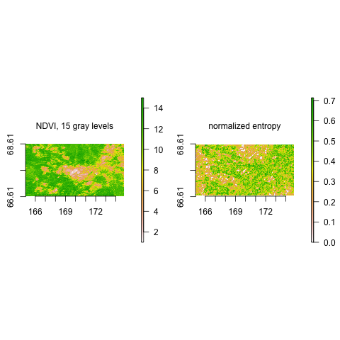
install.packages("StrucDiv")Calculate normalized entropy on Normalized Difference Vegetation Index (NDVI) data, which was binned to 15 gray levels (see data documentation). Scale is defined by window size length (WSL) 3, direct value neighbors are considered, and the direction-invariant version is employed.
ndvi.15gl <- raster(ndvi.15gl)
extent(ndvi.15gl) <-  c(165.0205, 174.8301, 66.62804, 68.61332)

entNorm <- strucDiv(ndvi.15gl, wsl = 5, dist = 1, angle = "all", fun = entropyNorm,
                  na.handling = na.pass)