The goal of patterncausality is to measure the causality in the complex system. The core of this algorithm is measure the strength of each causality status like positive, negative, and dark in the view of complex system, this method could be used for many different fields like financial market, ecosystem, medical diagnosis and so on.
This algorithm has a lot of advantages.
You can install the development version of patterncausality from GitHub with:
# install.packages("devtools")
devtools::install_github("skstavroglou/pattern-causality")We can import the existing data.
library(patterncausality)
#> Warning in fun(libname, pkgname): couldn't connect to display ":0"data(climate)
head(climate)
#> Date AO AAO NAO PNA
#> 1 1979-01-01 -2.2328 0.2088 -1.38 -0.69
#> 2 1979-02-01 -0.6967 0.3563 -0.67 -1.82
#> 3 1979-03-01 -0.8141 0.8992 0.78 0.38
#> 4 1979-04-01 -1.1568 0.6776 -1.71 0.09
#> 5 1979-05-01 -0.2501 0.7237 -1.03 1.35
#> 6 1979-06-01 0.9332 1.7000 1.60 -1.64This dataset contains 4 time series of climate index, we could use the patterncausality in this dataset.
Then we need to determine the E and
tao.
dataset <- climate[, -1] # remove the date column
parameter <- optimalParametersSearch(Emax = 5, tauMax = 5, metric = "euclidean", dataset = dataset)| Total | of which Positive | of which Negative | of which Dark | ||
|---|---|---|---|---|---|
| E = 2 | tau = 1 | 0.5543614 | 0.5519477 | 0.4474361 | 0.0006162144 |
| E = 2 | tau = 2 | 0.5727414 | 0.5736100 | 0.4232828 | 0.0031071596 |
| E = 2 | tau = 3 | 0.5711838 | 0.5469069 | 0.4513270 | 0.0017660870 |
| E = 3 | tau = 1 | 0.3305296 | 0.3457169 | 0.2470929 | 0.4071902523 |
| E = 3 | tau = 2 | 0.3500000 | 0.4037138 | 0.2547524 | 0.3415338782 |
| E = 3 | tau = 3 | 0.3570093 | 0.3657638 | 0.2690536 | 0.3651826225 |
Of course, we can also change the distance style to calculate the distance matrix.
After the parameters are confirmed, we could calculate the pattern causality.
X <- climate$AO
Y <- climate$AAO
pc <- PC.Mk.II.Lightweight(X, Y, E = 3, tau = 2, metric = "euclidean", h = 1, weighted = TRUE)
print(pc)
#>       total positive  negative     dark
#> 1 0.2841121 0.326087 0.2318841 0.442029
Then the percentage of each status will be showed below.
If we wonder the status in each time point, we can run the code.
X <- climate$AO
Y <- climate$AAO
detail <- PC.Mk.II.Full.Details(X, Y, E = 2, tau = 1, metric = "euclidean", h = 3, weighted = TRUE)
predict_status <- detail$spectrumOfCausalityPredicted
real_stattus <- detail$spectrumOfCausalityReal
Then the status series will be saved in predict_status
and real_status.
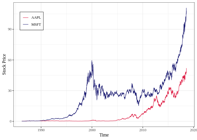
First of all, we can import the data of AAPL and MSFT.
data(stock)
head(stock)
#>            AAPL.Open AAPL.High AAPL.Low AAPL.Close AAPL.Volume AAPL.Adjusted
#> 1986-03-13  0.110491  0.111607 0.108817   0.110491   115964800    0.08527586
#> 1986-03-14  0.110491  0.117188 0.110491   0.116629   384854400    0.09001311
#> 1986-03-17  0.116071  0.116071 0.113281   0.116071   118720000    0.08958244
#> 1986-03-18  0.116071  0.121652 0.115513   0.119978   249356800    0.09259786
#> 1986-03-19  0.119978  0.121652 0.117746   0.118304   189884800    0.09130585
#> 1986-03-20  0.125000  0.132254 0.125000   0.126116   904131200    0.09733511
#>            MSFT.Open MSFT.High MSFT.Low MSFT.Close MSFT.Volume MSFT.Adjusted
#> 1986-03-13  0.088542  0.101563 0.088542   0.097222  1031788800    0.06005456
#> 1986-03-14  0.097222  0.102431 0.097222   0.100694   308160000    0.06219922
#> 1986-03-17  0.100694  0.103299 0.100694   0.102431   133171200    0.06327216
#> 1986-03-18  0.102431  0.103299 0.098958   0.099826    67766400    0.06166304
#> 1986-03-19  0.099826  0.100694 0.097222   0.098090    47894400    0.06059071
#> 1986-03-20  0.098090  0.098090 0.094618   0.095486    58435200    0.05898221
We can visualize this stock price.
#> Warning: A numeric `legend.position` argument in `theme()` was deprecated in ggplot2
#> 3.5.0.
#> ℹ Please use the `legend.position.inside` argument of `theme()` instead.
#> This warning is displayed once every 8 hours.
#> Call `lifecycle::last_lifecycle_warnings()` to see where this warning was
#> generated.
Then search the best parameters for the PC.
dataset <- stock
parameter <- optimalParametersSearch(Emax = 5, tauMax = 5, metric = "euclidean", dataset = dataset)
After that, calculate the causality of each status.
X <- stock$AAPL.Close
Y <- stock$MSFT.Close
pc <- PC.Mk.II.Lightweight(X, Y, E = 3, tau = 2, metric = "euclidean", h = 1, weighted = TRUE)
print(pc)
#>       total  positive  negative      dark
#> 1 0.2698665 0.3881279 0.1369863 0.4748858
Lastly we can also visualize this result.
library(ggplot2)
df = data.frame(
  name=stringr::str_to_title(c(colnames(pc))),
  val=as.vector(unlist(pc))
)

ggplot(df, aes(x=name, y=val, fill=name)) +
  geom_bar(stat="identity", alpha=.6, width=.4) +
  scale_fill_grey(start=0, end=0.8) +  # start and end define the range of grays
  labs(x='Status',y='Strength')+
  theme_bw(base_size = 12, base_family = "Times New Roman") +
  theme(legend.position="none", axis.text   = element_text(size = rel(0.8)),
                strip.text  = element_text(size = rel(0.8)))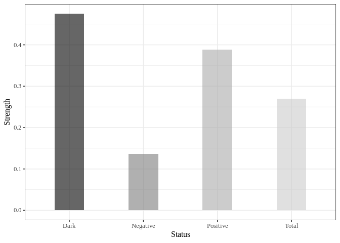
After calculating the causality, we can get the result here.
| Pairs | total | positive | negative | dark | Dataset |
|---|---|---|---|---|---|
| AAPL –> MSFT | 0.2698665 | 0.3881279 | 0.1369863 | 0.4748858 | stock |
| MSFT –> AAPL | 0.2759887 | 0.4075893 | 0.1388393 | 0.4535714 | stock |
| AO –> AAO | 0.2841121 | 0.326087 | 0.2318841 | 0.442029 | climate |
| AAO –> AO | 0.2803738 | 0.3602941 | 0.2647059 | 0.375 | climate |
| AO –> P | 0.3084112 | 0.1192053 | 0.4503311 | 0.4304636 | AUCO |
| P –> AO | 0.3308411 | 0.3374233 | 0.2515337 | 0.4110429 | AUCO |
Stavroglou, S. K., Pantelous, A. A., Stanley, H. E., & Zuev, K. M. (2019). Hidden interactions in financial markets. Proceedings of the National Academy of Sciences, 116(22), 10646-10651.
Stavroglou, S. K., Pantelous, A. A., Stanley, H. E., & Zuev, K. M. (2020). Unveiling causal interactions in complex systems. Proceedings of the National Academy of Sciences, 117(14), 7599-7605.
Stavroglou, S. K., Ayyub, B. M., Kallinterakis, V., Pantelous, A. A., & Stanley, H. E. (2021). A novel causal risk‐based decision‐making methodology: The case of coronavirus. Risk Analysis, 41(5), 814-830.
Stavroglou, S. K., Pantelous, A. A., Ayyub, B. M., Lambert, J. H., Hall, J. W., & Stanley, H. E. (2023). Prometheus Framework for Public Policy Decisions on Environmental Health Risks. Available at SSRN 4526256.