
AeroSampleR is an R package to help estimate the fraction of aerosol particles that make their way through an air sampling system.
You can install the released version of AeroSampleR from CRAN with:
install.packages("AeroSampleR")Or install the development version from GitHub:
# install.packages("devtools")
devtools::install_github("markhogue/AeroSampleR")Air sampling systems are in use in nuclear facilities and other facilities that have a potential for hazardous airborne particles. Ambient air is drawn in at one end of a system through a probe, and directed through tubing components (e.g. straight lines, bends).
As the air sample progresses through the system, some particles deposit along the way on the inside of the tubing. How much is lost depends on a number of factors, such as particle size, system length, bend diameter, etc.
AeroSampleR relies on the concept of aerodynamic median activity diameter (AMAD), which accounts for particle density and shape, leaving equivalent spherical water droplets as the modeling targets.
Efficiency functions are based predominantly on testing with aerosol particles through stainless steel tubing. These models are only valid for clean systems. If a system is coated on the inside with years of material accumulation, or if the system is unprotected from environmental factors that could produce interior condensation, then there should be no expectation that the models will produce a realistic result.
At this time, only relatively simple systems can be modeled with AeroSampleR. Components evaluated include:
Not included:
The following is an example evaluation of a simple sampling system:
Initiate a table of data populated with particle diameters
df <- particle_dist() # no entries = default particle sizes
#>
#>
#>
#> _mean_ diameter for AMAD (median activity) =  0.9427043
The mean is shown above. The mean is used to derive the particle
distribution using the stats::dlnorm function. The mean has
to first be derived for the lognormal particle distribution with the
median and standard deviation that are used as arguments to the
particle_dist function.
Add the system parameters
params <- set_params_1("D_tube" = 2.54, # 1 inch diameter
                       "Q_lpm" = 100, # ~3.53 cfm
                       "T_C" = 25, # 77 F
                       "P_kPa" = 101.325) # Atmospheric pressure at sea level
Add particle size dependent parameters
df <- set_params_2(df, params)Start the system with a probe oriented upwards (“u”)
df <- probe_eff(df, params, orient = "u")Our system has a 90 degree bend after the probe. We’re using the Zhang model
df <- bend_eff(df,
               params,
               method = "Zhang",
               bend_angle = 45,
               bend_radius = 0.1,
               elnum = 2) #each element after the probe should be numbered
Next, our system has a straight line to the detector
df <- tube_eff(df,
               params,
               L = 1, # 1 meter
               angle_to_horiz = 0,
               elnum = 3)
That’s the whole system. As we added elements, our table of data added columns. Let’s look under the hood at the data frame (df) we made. We’ll look at the end where the discrete values start.
print.data.frame(df[1001:1003, ], digits = 2, row.names = FALSE) #formatted to fit
#>  D_p probs     dist C_c    v_ts    Re_p     Stk eff_probe eff_bend_2 eff_tube_3
#>    1     1 discrete 1.2 3.6e-05 2.3e-06 0.00094         1       1.00       1.00
#>    5     1 discrete 1.0 7.7e-04 2.5e-04 0.02023         1       0.98       0.99
#>   10     1 discrete 1.0 3.0e-03 1.9e-03 0.07954         1       0.93       0.92
Let’s evaluate - discrete first
 report_basic(df, params, "discrete")
#> System Parameters
#> All values in MKS units, except noted
#> Notes: D_tube is in m.
#> Q_lpm is system flow in liters per minute.
#> velocity_air is the derived air flow velocity in meters per second.T_K is system temperature in Kelvin.
#> P_kPa is system pressure in kiloPascals.
#> Re is the system Reynolds number, a measure of turbulence.
#>   microns   sys_eff
#> 1       1 0.9987645
#> 2       5 0.9712557
#> 3      10 0.8545854
Plot
report_plots(df, "discrete")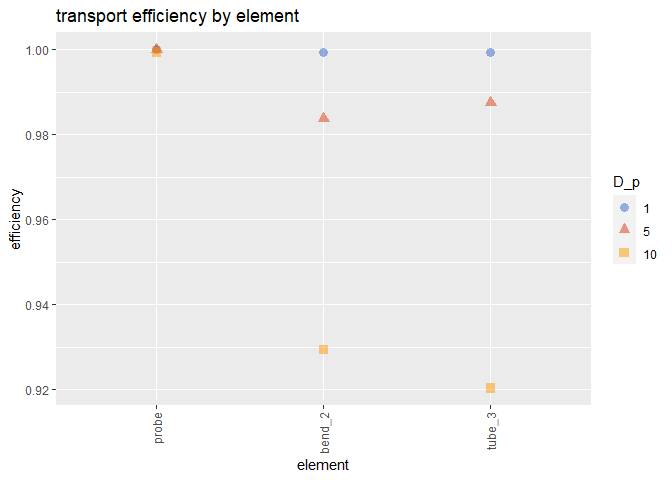
Logarithmic report
report_basic(df, params, "log")
#> System Parameters
#> All values in MKS units, except noted
#> Notes: D_tube is in m.
#> Q_lpm is system flow in liters per minute.
#> velocity_air is the derived air flow velocity in meters per second.T_K is system temperature in Kelvin.
#> P_kPa is system pressure in kiloPascals.
#> Re is the system Reynolds number, a measure of turbulence.
#>   eff_mass_weighted
#> 1         0.8444339
Plot
report_plots(df, "log")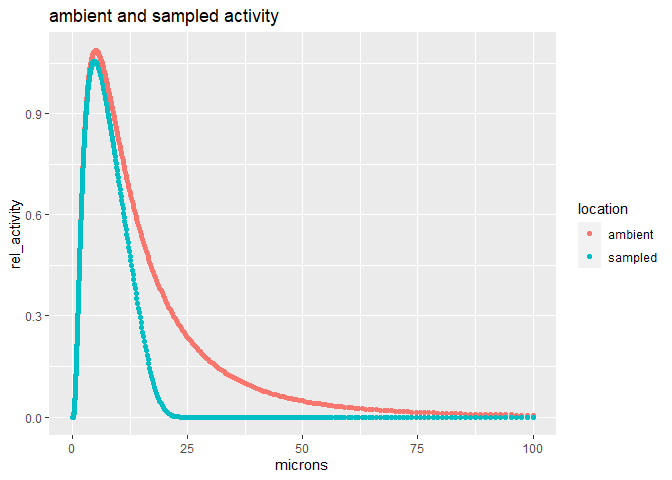
A sample of the logarithmic data
df_log <- report_log_mass(df)[600:620, ]
print.data.frame(df_log, digits = 3, row.names = FALSE)
#>  microns probs bin_eff amb_mass sampled_mass bin_frac_lost total_frac_lost
#>    0.754 0.560   0.999    0.126        0.126      0.000792        4.88e-07
#>    0.763 0.555   0.999    0.129        0.129      0.000806        5.11e-07
#>    0.773 0.550   0.999    0.133        0.133      0.000820        5.35e-07
#>    0.782 0.545   0.999    0.137        0.137      0.000835        5.59e-07
#>    0.792 0.540   0.999    0.140        0.140      0.000851        5.85e-07
#>    0.802 0.535   0.999    0.144        0.144      0.000866        6.12e-07
#>    0.812 0.529   0.999    0.148        0.148      0.000882        6.41e-07
#>    0.822 0.524   0.999    0.152        0.152      0.000899        6.70e-07
#>    0.832 0.519   0.999    0.156        0.156      0.000916        7.01e-07
#>    0.842 0.513   0.999    0.160        0.160      0.000934        7.34e-07
#>    0.852 0.508   0.999    0.165        0.164      0.000952        7.67e-07
#>    0.863 0.502   0.999    0.169        0.169      0.000970        8.03e-07
#>    0.873 0.497   0.999    0.173        0.173      0.000989        8.40e-07
#>    0.884 0.491   0.999    0.178        0.178      0.001008        8.78e-07
#>    0.895 0.486   0.999    0.182        0.182      0.001028        9.19e-07
#>    0.906 0.480   0.999    0.187        0.187      0.001049        9.61e-07
#>    0.917 0.475   0.999    0.192        0.191      0.001070        1.00e-06
#>    0.928 0.469   0.999    0.196        0.196      0.001091        1.05e-06
#>    0.940 0.463   0.999    0.201        0.201      0.001114        1.10e-06
#>    0.951 0.458   0.999    0.206        0.206      0.001136        1.15e-06
#>    0.963 0.452   0.999    0.211        0.211      0.001160        1.20e-06