AlleleShift is an R package to predict and visualize
population-level changes in allele frequencies.
The following manuscript provides details on the methods used by the package: Kindt R. 2021 (in prep.) AlleleShift: An R package to predict and visualize population-level changes in allele frequencies in response to climate change.
To install from CRAN, use:
install.packages('AlleleShift')The package can be installed from github via:
# install.packages('devtools')
devtools::install_github('RoelandKindt/AlleleShift')library(BiodiversityR) # also loads vegan
library(poppr) # also loads adegenet
library(ggplot2)
library(ggsci)
library(ggforce)
library(dplyr)
library(ggrepel)
library(patchwork)
library(GGally)
library(mgcv)
library(ggmap)
library(gggibbous)
library(gganimate)
library(AlleleShift)The following script is also available from the documentation of the ‘count.model’ function.
Input data ‘Poptri.baseline.env’ and ‘Poptri.future.env’ document bioclimatic conditions for populations in baseline and future climates. ‘Poptri.genind’ is information on allele counts of individuals in the ‘adegenet::genind’ format (note that packages ‘adegenet’ and ‘poppr’ offer various methods of importing data from other applications).
# 1. Reduce the number of explanatory variables
data(Poptri.baseline.env)
data(Poptri.future.env)
VIF.select <- VIF.subset(Poptri.baseline.env,
keep=c("MAT", "CMI"),
cor.plot=TRUE)
#> Step 1: Keeping these vars:
#> [1] "MAT" "CMI" "TD" "MSP" "AHM" "SHM" "DD.0" "bFFP"
#> [9] "PAS" "Eref" "CMD" "cmiJJA" "PPT_sm" "Tmax07"
#>
#> Variance inflation (package: car)
#> MAT TD MSP AHM SHM DD.0 bFFP
#> 1956.71402 55.35151 325.04715 258.27807 199.03579 383.71475 208.48116
#> PAS Eref CMD CMI cmiJJA PPT_sm Tmax07
#> 418.39278 509.80399 702.97284 729.58048 2108.47844 1221.60927 404.91923
#>
#> VIF directly calculated from linear model with focal numeric variable as response
#> cmiJJA MAT PPT_sm CMI CMD Eref PAS
#> 2108.47844 1956.71402 1221.60927 729.58048 702.97284 509.80399 418.39278
#> Tmax07 DD.0 MSP AHM bFFP SHM TD
#> 404.91923 383.71475 325.04715 258.27807 208.48116 199.03579 55.35151
#>
#> Variance inflation (package: car)
#> MAT TD MSP AHM SHM DD.0 bFFP
#> 1152.51188 51.00442 280.39905 196.06676 189.87780 289.82940 177.01912
#> PAS Eref CMD CMI PPT_sm Tmax07
#> 373.46930 302.59709 652.89020 548.59673 527.99218 186.61090
#>
#> VIF directly calculated from linear model with focal numeric variable as response
#> MAT CMD CMI PPT_sm PAS Eref DD.0
#> 1152.51188 652.89020 548.59673 527.99218 373.46930 302.59709 289.82940
#> MSP AHM SHM Tmax07 bFFP TD
#> 280.39905 196.06676 189.87780 186.61090 177.01912 51.00442
#>
#> Variance inflation (package: car)
#> MAT TD MSP AHM SHM DD.0 bFFP PAS
#> 775.21530 48.40917 275.40371 179.50626 90.11375 260.05137 146.29625 368.40367
#> Eref CMI PPT_sm Tmax07
#> 102.83305 545.11114 394.89879 180.19703
#>
#> VIF directly calculated from linear model with focal numeric variable as response
#> MAT CMI PPT_sm PAS MSP DD.0 Tmax07 AHM
#> 775.21530 545.11114 394.89879 368.40367 275.40371 260.05137 180.19703 179.50626
#> bFFP Eref SHM TD
#> 146.29625 102.83305 90.11375 48.40917
#>
#> Variance inflation (package: car)
#> MAT TD MSP AHM SHM DD.0 bFFP PAS
#> 528.61146 32.01349 145.93063 78.09567 53.38943 222.17330 145.00874 188.09374
#> Eref CMI Tmax07
#> 102.40225 306.50400 111.10074
#>
#> VIF directly calculated from linear model with focal numeric variable as response
#> MAT CMI DD.0 PAS MSP bFFP Tmax07 Eref
#> 528.61146 306.50400 222.17330 188.09374 145.93063 145.00874 111.10074 102.40225
#> AHM SHM TD
#> 78.09567 53.38943 32.01349
#>
#> Variance inflation (package: car)
#> MAT TD MSP AHM SHM bFFP PAS Eref
#> 291.46937 30.38197 64.59840 46.78232 37.94467 45.37584 45.57930 99.66232
#> CMI Tmax07
#> 93.58775 109.62229
#>
#> VIF directly calculated from linear model with focal numeric variable as response
#> MAT Tmax07 Eref CMI MSP AHM PAS bFFP
#> 291.46937 109.62229 99.66232 93.58775 64.59840 46.78232 45.57930 45.37584
#> SHM TD
#> 37.94467 30.38197
#>
#> Variance inflation (package: car)
#> MAT TD MSP AHM SHM bFFP PAS
#> 237.300281 4.513064 62.232526 46.486704 37.871152 44.616210 44.930713
#> Eref CMI
#> 33.411744 85.667431
#>
#> VIF directly calculated from linear model with focal numeric variable as response
#> MAT CMI MSP AHM PAS bFFP SHM
#> 237.300281 85.667431 62.232526 46.486704 44.930713 44.616210 37.871152
#> Eref TD
#> 33.411744 4.513064
#>
#> Variance inflation (package: car)
#> MAT TD AHM SHM bFFP PAS Eref
#> 218.240423 4.170754 25.872364 5.680412 43.733182 39.989330 32.625175
#> CMI
#> 27.162467
#>
#> VIF directly calculated from linear model with focal numeric variable as response
#> MAT bFFP PAS Eref CMI AHM SHM
#> 218.240423 43.733182 39.989330 32.625175 27.162467 25.872364 5.680412
#> TD
#> 4.170754
#>
#> Variance inflation (package: car)
#> MAT TD AHM SHM PAS Eref CMI
#> 56.168045 4.154401 24.524555 5.474406 31.877700 13.105090 22.368212
#>
#> VIF directly calculated from linear model with focal numeric variable as response
#> MAT PAS AHM CMI Eref SHM TD
#> 56.168045 31.877700 24.524555 22.368212 13.105090 5.474406 4.154401
#>
#> Variance inflation (package: car)
#> MAT TD AHM SHM Eref CMI
#> 8.713339 4.003336 19.299959 5.465614 9.025702 14.431931
#>
#> VIF directly calculated from linear model with focal numeric variable as response
#> AHM CMI Eref MAT SHM TD
#> 19.299959 14.431931 9.025702 8.713339 5.465614 4.003336
#>
#> Summary of VIF selection process:
#> MAT TD MSP AHM SHM DD.0 bFFP
#> step_1 1956.714025 55.351511 325.04715 258.27807 199.035789 383.7148 208.48116
#> step_2 1152.511883 51.004421 280.39905 196.06676 189.877801 289.8294 177.01912
#> step_3 775.215296 48.409171 275.40371 179.50626 90.113750 260.0514 146.29625
#> step_4 528.611459 32.013493 145.93063 78.09567 53.389431 222.1733 145.00874
#> step_5 291.469373 30.381965 64.59840 46.78232 37.944668 NA 45.37584
#> step_6 237.300281 4.513064 62.23253 46.48670 37.871152 NA 44.61621
#> step_7 218.240423 4.170754 NA 25.87236 5.680412 NA 43.73318
#> step_8 56.168045 4.154401 NA 24.52456 5.474406 NA NA
#> step_9 8.713339 4.003336 NA 19.29996 5.465614 NA NA
#> PAS Eref CMD CMI cmiJJA PPT_sm Tmax07
#> step_1 418.39278 509.803994 702.9728 729.58048 2108.478 1221.6093 404.9192
#> step_2 373.46930 302.597094 652.8902 548.59673 NA 527.9922 186.6109
#> step_3 368.40367 102.833047 NA 545.11114 NA 394.8988 180.1970
#> step_4 188.09374 102.402249 NA 306.50400 NA NA 111.1007
#> step_5 45.57930 99.662321 NA 93.58775 NA NA 109.6223
#> step_6 44.93071 33.411744 NA 85.66743 NA NA NA
#> step_7 39.98933 32.625175 NA 27.16247 NA NA NA
#> step_8 31.87770 13.105090 NA 22.36821 NA NA NA
#> step_9 NA 9.025702 NA 14.43193 NA NA NA
#>
#> Final selection of variables:
#> [1] "AHM" "CMI" "Eref" "MAT" "SHM" "TD"
VIF.select$VIF$vars.included
#> [1] "AHM" "CMI" "Eref" "MAT" "SHM" "TD"
baseline.env <- Poptri.baseline.env[, VIF.select$VIF$vars.included]
summary(baseline.env)
#> AHM CMI Eref MAT
#> Min. : 5.50 Min. : 29.0 Min. :455.0 Min. : 1.690
#> 1st Qu.: 8.45 1st Qu.: 55.5 1st Qu.:602.0 1st Qu.: 5.620
#> Median :10.80 Median : 97.0 Median :675.0 Median : 8.980
#> Mean :12.06 Mean :109.5 Mean :680.9 Mean : 7.903
#> 3rd Qu.:16.80 3rd Qu.:150.5 3rd Qu.:773.5 3rd Qu.:10.045
#> Max. :19.50 Max. :232.0 Max. :920.0 Max. :11.290
#> SHM TD
#> Min. : 23.50 Min. :13.90
#> 1st Qu.: 38.45 1st Qu.:14.25
#> Median : 50.20 Median :15.30
#> Mean : 56.53 Mean :16.11
#> 3rd Qu.: 74.40 3rd Qu.:17.60
#> Max. :102.90 Max. :20.10
future.env <- Poptri.future.env[, VIF.select$VIF$vars.included]
# 2. Create the genpop object
data(Poptri.genind)
Poptri.genpop <- adegenet::genind2genpop(Poptri.genind)
#>
#> Converting data from a genind to a genpop object...
#>
#> ...done.
# Get to know the populations and the alleles
poppr::poppr(Poptri.genind)
#> Pop N MLG eMLG SE H G lambda E.5 Hexp Ia
#> 1 Chilliwack 38 14 5.67 1.244 1.972 3.97 0.748 0.480 0.168 0.29948
#> 2 Columbia 180 31 6.69 1.276 2.634 8.17 0.878 0.555 0.219 0.03214
#> 3 Dean 7 4 4.00 0.000 1.352 3.77 0.735 0.967 0.145 -0.16667
#> 4 Harrison 22 10 5.87 1.093 1.855 4.10 0.756 0.575 0.191 0.06387
#> 5 Homathko 9 7 7.00 0.000 1.831 5.40 0.815 0.840 0.182 -0.17703
#> 6 Kitimat 8 4 4.00 0.000 1.321 3.56 0.719 0.930 0.127 -0.13245
#> 7 Klinaklini 8 5 5.00 0.000 1.494 4.00 0.750 0.868 0.155 -0.41248
#> 8 Nisqually 14 7 5.51 0.830 1.567 3.38 0.704 0.627 0.157 0.00845
#> 9 Nooksack 26 11 6.44 1.072 2.124 6.76 0.852 0.782 0.211 0.05709
#> 10 Olympic_Penninsula 5 3 3.00 0.000 0.950 2.27 0.560 0.802 0.191 -0.25000
#> 11 Puyallup 186 29 6.03 1.303 2.396 5.81 0.828 0.482 0.178 -0.02222
#> 12 Salmon 11 7 6.64 0.481 1.846 5.76 0.826 0.892 0.193 -0.19978
#> 13 Skagit 163 20 5.41 1.268 2.102 4.72 0.788 0.518 0.168 -0.01194
#> 14 Skwawka 14 6 5.29 0.656 1.631 4.45 0.776 0.841 0.160 -0.04804
#> 15 Skykomish 156 31 6.97 1.249 2.730 9.26 0.892 0.576 0.233 0.07931
#> 16 Squamish 14 10 7.86 0.802 2.206 8.17 0.878 0.887 0.205 -0.28884
#> 17 Tahoe 12 9 7.82 0.649 2.095 7.20 0.861 0.870 0.293 -0.11481
#> 18 Vancouver I. East 12 4 3.50 0.584 0.837 1.71 0.417 0.546 0.107 0.48361
#> 19 Willamette 17 10 6.65 1.016 2.007 5.45 0.817 0.691 0.246 0.11902
#> 20 Total 902 59 6.38 1.323 2.663 6.93 0.856 0.445 0.200 0.03621
#> rbarD File
#> 1 0.08166 Poptri.genind
#> 2 0.00883 Poptri.genind
#> 3 -0.16667 Poptri.genind
#> 4 0.02067 Poptri.genind
#> 5 -0.04770 Poptri.genind
#> 6 -0.14222 Poptri.genind
#> 7 -0.21444 Poptri.genind
#> 8 0.00445 Poptri.genind
#> 9 0.01646 Poptri.genind
#> 10 -0.25000 Poptri.genind
#> 11 -0.00606 Poptri.genind
#> 12 -0.07663 Poptri.genind
#> 13 -0.00373 Poptri.genind
#> 14 -0.01849 Poptri.genind
#> 15 0.02249 Poptri.genind
#> 16 -0.08273 Poptri.genind
#> 17 -0.03060 Poptri.genind
#> 18 0.27081 Poptri.genind
#> 19 0.04139 Poptri.genind
#> 20 0.00998 Poptri.genind
adegenet::makefreq(Poptri.genpop)
#>
#> Finding allelic frequencies from a genpop object...
#>
#> ...done.
#> X01_10838495.1 X01_10838495.2 X01_16628872.1 X01_16628872.2
#> Chilliwack 0.10526316 0.8947368 0.19736842 0.8026316
#> Columbia 0.23055556 0.7694444 0.20000000 0.8000000
#> Dean 0.21428571 0.7857143 0.00000000 1.0000000
#> Harrison 0.15909091 0.8409091 0.25000000 0.7500000
#> Homathko 0.05555556 0.9444444 0.22222222 0.7777778
#> Kitimat 0.25000000 0.7500000 0.12500000 0.8750000
#> Klinaklini 0.06250000 0.9375000 0.43750000 0.5625000
#> Nisqually 0.10714286 0.8928571 0.25000000 0.7500000
#> Nooksack 0.17307692 0.8269231 0.26923077 0.7307692
#> Olympic_Penninsula 0.50000000 0.5000000 0.10000000 0.9000000
#> Puyallup 0.17204301 0.8279570 0.16935484 0.8306452
#> Salmon 0.04545455 0.9545455 0.27272727 0.7272727
#> Skagit 0.23619632 0.7638037 0.18098160 0.8190184
#> Skwawka 0.03571429 0.9642857 0.32142857 0.6785714
#> Skykomish 0.20192308 0.7980769 0.31410256 0.6858974
#> Squamish 0.28571429 0.7142857 0.25000000 0.7500000
#> Tahoe 0.62500000 0.3750000 0.08333333 0.9166667
#> Vancouver I. East 0.16666667 0.8333333 0.00000000 1.0000000
#> Willamette 0.35294118 0.6470588 0.20588235 0.7941176
#> X01_23799134.1 X01_23799134.2 X01_38900650.1 X01_38900650.2
#> Chilliwack 0.06578947 0.9342105 0.05263158 0.9473684
#> Columbia 0.10833333 0.8916667 0.06944444 0.9305556
#> Dean 0.00000000 1.0000000 0.21428571 0.7857143
#> Harrison 0.11363636 0.8863636 0.02272727 0.9772727
#> Homathko 0.05555556 0.9444444 0.05555556 0.9444444
#> Kitimat 0.00000000 1.0000000 0.00000000 1.0000000
#> Klinaklini 0.00000000 1.0000000 0.00000000 1.0000000
#> Nisqually 0.00000000 1.0000000 0.00000000 1.0000000
#> Nooksack 0.01923077 0.9807692 0.07692308 0.9230769
#> Olympic_Penninsula 0.00000000 1.0000000 0.00000000 1.0000000
#> Puyallup 0.04569892 0.9543011 0.05107527 0.9489247
#> Salmon 0.00000000 1.0000000 0.04545455 0.9545455
#> Skagit 0.03987730 0.9601227 0.01840491 0.9815951
#> Skwawka 0.07142857 0.9285714 0.00000000 1.0000000
#> Skykomish 0.11217949 0.8878205 0.03525641 0.9647436
#> Squamish 0.03571429 0.9642857 0.03571429 0.9642857
#> Tahoe 0.04166667 0.9583333 0.41666667 0.5833333
#> Vancouver I. East 0.00000000 1.0000000 0.08333333 0.9166667
#> Willamette 0.00000000 1.0000000 0.14705882 0.8529412
#> X01_41284594.1 X01_41284594.2
#> Chilliwack 0.05263158 0.9473684
#> Columbia 0.05000000 0.9500000
#> Dean 0.00000000 1.0000000
#> Harrison 0.02272727 0.9772727
#> Homathko 0.11111111 0.8888889
#> Kitimat 0.00000000 1.0000000
#> Klinaklini 0.06250000 0.9375000
#> Nisqually 0.10714286 0.8928571
#> Nooksack 0.09615385 0.9038462
#> Olympic_Penninsula 0.10000000 0.9000000
#> Puyallup 0.07526882 0.9247312
#> Salmon 0.22727273 0.7727273
#> Skagit 0.03374233 0.9662577
#> Skwawka 0.07142857 0.9285714
#> Skykomish 0.07692308 0.9230769
#> Squamish 0.03571429 0.9642857
#> Tahoe 0.12500000 0.8750000
#> Vancouver I. East 0.04166667 0.9583333
#> Willamette 0.08823529 0.9117647
# 3. Calibrate the models
# Note that the ordistep procedure is not needed
Poptri.count.model <- count.model(Poptri.genpop,
env.data=baseline.env,
ordistep=TRUE)
#>
#> Finding allelic frequencies from a genpop object...
#>
#> ...done.
#>
#>
#> Call:
#> rda(formula = gen.comm.b ~ AHM + CMI + Eref + MAT + SHM + TD, data = env.data)
#>
#> Partitioning of variance:
#> Inertia Proportion
#> Total 13675 1.0000
#> Constrained 6841 0.5002
#> Unconstrained 6834 0.4998
#>
#> Eigenvalues, and their contribution to the variance
#>
#> Importance of components:
#> RDA1 RDA2 RDA3 RDA4 RDA5
#> Eigenvalue 5203.4791 893.09032 489.16133 249.89783 5.3852777
#> Proportion Explained 0.3805 0.06531 0.03577 0.01827 0.0003938
#> Cumulative Proportion 0.3805 0.44580 0.48157 0.49985 0.5002410
#> PC1 PC2 PC3 PC4 PC5
#> Eigenvalue 4597.4331 1443.5788 458.75766 243.85111 90.80236
#> Proportion Explained 0.3362 0.1056 0.03355 0.01783 0.00664
#> Cumulative Proportion 0.8364 0.9420 0.97553 0.99336 1.00000
#>
#> Accumulated constrained eigenvalues
#> Importance of components:
#> RDA1 RDA2 RDA3 RDA4 RDA5
#> Eigenvalue 5203.4791 893.0903 489.1613 249.89783 5.3852777
#> Proportion Explained 0.7606 0.1305 0.0715 0.03653 0.0007872
#> Cumulative Proportion 0.7606 0.8912 0.9627 0.99921 1.0000000
#>
#> Scaling 2 for species and site scores
#> * Species are scaled proportional to eigenvalues
#> * Sites are unscaled: weighted dispersion equal on all dimensions
#> * General scaling constant of scores: 22.27427
#>
#>
#> Species scores
#>
#> RDA1 RDA2 RDA3 RDA4 RDA5 PC1
#> X01_10838495.1 7.7466 -0.7259 -1.69114 0.187490 -0.01266 6.28376
#> X01_10838495.2 -7.7466 0.7259 1.69114 -0.187490 0.01266 -6.28376
#> X01_16628872.1 -2.2584 2.5545 -1.43674 0.084325 -0.17373 -5.83911
#> X01_16628872.2 2.2584 -2.5545 1.43674 -0.084325 0.17373 5.83911
#> X01_23799134.1 -0.4671 1.9706 -0.83990 -0.001968 0.25745 0.03723
#> X01_23799134.2 0.4671 -1.9706 0.83990 0.001968 -0.25745 -0.03723
#> X01_38900650.1 5.2463 2.2731 1.80100 0.256469 -0.03033 2.62821
#> X01_38900650.2 -5.2463 -2.2731 -1.80100 -0.256469 0.03033 -2.62821
#> X01_41284594.1 1.2400 0.3130 0.01204 -2.103589 -0.01203 -1.70511
#> X01_41284594.2 -1.2400 -0.3130 -0.01204 2.103589 0.01203 1.70511
#>
#>
#> Site scores (weighted sums of species scores)
#>
#> RDA1 RDA2 RDA3 RDA4 RDA5 PC1
#> Chilliwack -3.6364 1.6841 5.3973 1.4271 39.264 2.5785
#> Columbia 0.4218 2.5336 -3.8742 4.1743 71.373 0.4335
#> Dean 4.6551 -6.6279 24.0513 14.2372 83.823 8.0787
#> Harrison -3.3140 4.2633 -5.5469 7.1447 53.583 -2.0779
#> Homathko -5.0101 4.0804 8.0351 -9.1976 12.167 -4.4760
#> Kitimat 0.2023 -11.0757 -2.1893 11.1417 24.158 6.4103
#> Klinaklini -7.9981 10.8293 -7.6871 -0.3698 -176.410 -12.6881
#> Nisqually -4.7481 -0.5922 0.4640 -8.6869 -56.562 -7.2177
#> Nooksack -1.4050 4.2429 -0.2436 -4.0265 -61.991 1.2854
#> Olympic_Penninsula 8.5460 -15.9908 -18.3575 -2.4474 24.067 4.1194
#> Puyallup -1.2328 -1.8999 2.9514 -1.6765 34.025 1.7945
#> Salmon -5.3069 5.0051 6.9613 -29.2596 -79.379 -6.6457
#> Skagit -0.2454 -4.5544 -4.5800 5.8729 23.210 5.9223
#> Skwawka -7.8707 7.7636 -1.3073 -3.1379 -28.712 -4.6465
#> Skykomish -2.0503 8.2869 -11.4201 -0.8444 3.752 0.6351
#> Squamish 1.0273 -0.6021 -10.7934 7.1369 -31.007 1.5425
#> Tahoe 21.1711 4.7608 3.7894 3.8075 20.644 4.3325
#> Vancouver I. East 0.6973 -12.3697 17.5610 3.5557 99.335 1.0511
#> Willamette 6.0970 0.2625 -3.2114 1.1486 -55.342 -0.4317
#>
#>
#> Site constraints (linear combinations of constraining variables)
#>
#> RDA1 RDA2 RDA3 RDA4 RDA5 PC1
#> Chilliwack -5.3411 2.94631 -5.73690 -1.2669 3.6318 2.5785
#> Columbia 1.0348 1.48239 -4.35834 -1.9144 -1.5967 0.4335
#> Dean -0.7121 3.05536 13.59960 5.7383 -2.3972 8.0787
#> Harrison -0.6115 4.57450 -6.67046 12.7199 1.7520 -2.0779
#> Homathko -0.2101 4.51571 2.95659 0.1637 3.7693 -4.4760
#> Kitimat -5.7357 -7.72450 0.08812 2.8441 6.3705 6.4103
#> Klinaklini 0.9827 -2.48137 3.56265 6.7122 -7.5810 -12.6881
#> Nisqually 1.1218 -6.23684 -1.27479 0.7219 -0.9320 -7.2177
#> Nooksack -3.6818 3.17251 -4.89865 -2.9837 -3.8484 1.2854
#> Olympic_Penninsula 5.1563 -8.68730 -3.34262 -4.1673 0.8657 4.1194
#> Puyallup -2.4480 -0.01102 -0.54619 0.1670 -4.9542 1.7945
#> Salmon -1.1061 -0.60968 4.52845 -8.3433 -0.9208 -6.6457
#> Skagit -5.9406 -1.76614 0.27739 1.5322 -6.8831 5.9223
#> Skwawka -4.4370 1.80687 6.44400 -4.1364 14.0686 -4.6465
#> Skykomish -1.9900 10.49790 -2.02179 -9.1465 -5.7696 0.6351
#> Squamish -1.1546 0.32081 1.41105 4.4112 0.9792 1.5425
#> Tahoe 16.7611 4.67546 3.53694 -0.3315 1.2278 4.3325
#> Vancouver I. East 2.2338 -10.24318 1.07117 -4.5355 -3.0133 1.0511
#> Willamette 6.0779 0.71222 -8.62622 1.8151 5.2313 -0.4317
#>
#>
#> Biplot scores for constraining variables
#>
#> RDA1 RDA2 RDA3 RDA4 RDA5 PC1
#> AHM 0.13353 -0.29604 -0.5719 -0.16042 -0.4093 0
#> CMI -0.31497 0.20319 0.5713 0.04335 0.5768 0
#> Eref 0.29012 0.03393 -0.7039 -0.35686 -0.1588 0
#> MAT -0.07412 -0.21901 -0.7120 -0.54165 -0.1552 0
#> SHM 0.63769 -0.32011 -0.5075 -0.10019 -0.1988 0
#> TD -0.18759 0.19007 0.3043 0.67274 0.4208 0
#>
#> Permutation test for rda under reduced model
#> Permutation: free
#> Number of permutations: 99
#>
#> Model: rda(formula = gen.comm.b ~ AHM + CMI + Eref + MAT + SHM + TD, data = env.data)
#> Df Variance F Pr(>F)
#> Model 6 6841.0 2.0019 0.08 .
#> Residual 12 6834.4
#> ---
#> Signif. codes: 0 '***' 0.001 '**' 0.01 '*' 0.05 '.' 0.1 ' ' 1
#> Permutation test for rda under reduced model
#> Terms added sequentially (first to last)
#> Permutation: free
#> Number of permutations: 99
#>
#> Model: rda(formula = gen.comm.b ~ AHM + CMI + Eref + MAT + SHM + TD, data = env.data)
#> Df Variance F Pr(>F)
#> AHM 1 338.4 0.5942 0.58
#> CMI 1 1803.1 3.1659 0.07 .
#> Eref 1 1054.0 1.8507 0.14
#> MAT 1 872.8 1.5325 0.20
#> SHM 1 2259.1 3.9666 0.03 *
#> TD 1 513.5 0.9017 0.35
#> Residual 12 6834.4
#> ---
#> Signif. codes: 0 '***' 0.001 '**' 0.01 '*' 0.05 '.' 0.1 ' ' 1
#> Permutation test for rda under reduced model
#> Marginal effects of terms
#> Permutation: free
#> Number of permutations: 99
#>
#> Model: rda(formula = gen.comm.b ~ AHM + CMI + Eref + MAT + SHM + TD, data = env.data)
#> Df Variance F Pr(>F)
#> AHM 1 680.0 1.1940 0.32
#> CMI 1 135.1 0.2373 0.86
#> Eref 1 762.5 1.3388 0.27
#> MAT 1 538.0 0.9447 0.36
#> SHM 1 2141.2 3.7595 0.04 *
#> TD 1 513.5 0.9017 0.23
#> Residual 12 6834.4
#> ---
#> Signif. codes: 0 '***' 0.001 '**' 0.01 '*' 0.05 '.' 0.1 ' ' 1
#>
#> Start: gen.comm.b ~ 1
#>
#> Df AIC F Pr(>F)
#> + SHM 1 180.36 3.5025 0.040 *
#> + Eref 1 182.90 0.9356 0.315
#> + CMI 1 182.90 0.9379 0.405
#> + TD 1 183.39 0.4790 0.630
#> + MAT 1 183.36 0.5027 0.670
#> + AHM 1 183.44 0.4313 0.670
#> ---
#> Signif. codes: 0 '***' 0.001 '**' 0.01 '*' 0.05 '.' 0.1 ' ' 1
#>
#> Step: gen.comm.b ~ SHM
#>
#> Df AIC F Pr(>F)
#> - SHM 1 181.92 3.5025 0.045 *
#> ---
#> Signif. codes: 0 '***' 0.001 '**' 0.01 '*' 0.05 '.' 0.1 ' ' 1
#>
#> Df AIC F Pr(>F)
#> + MAT 1 178.52 3.5833 0.030 *
#> + AHM 1 177.28 4.9039 0.040 *
#> + Eref 1 180.08 2.0396 0.105
#> + CMI 1 180.18 1.9444 0.165
#> + TD 1 181.03 1.1544 0.330
#> ---
#> Signif. codes: 0 '***' 0.001 '**' 0.01 '*' 0.05 '.' 0.1 ' ' 1
#>
#> Step: gen.comm.b ~ SHM + MAT
#>
#> Df AIC F Pr(>F)
#> - MAT 1 180.36 3.5833 0.035 *
#> - SHM 1 183.36 6.9396 0.010 **
#> ---
#> Signif. codes: 0 '***' 0.001 '**' 0.01 '*' 0.05 '.' 0.1 ' ' 1
#>
#> Df AIC F Pr(>F)
#> + AHM 1 178.56 1.6263 0.215
#> + Eref 1 178.70 1.5047 0.220
#> + CMI 1 179.68 0.6724 0.540
#> + TD 1 179.79 0.5843 0.620
#>
#> Reduced model:
#> Permutation test for rda under reduced model
#> Permutation: free
#> Number of permutations: 99
#>
#> Model: rda(formula = gen.comm.b ~ SHM + MAT, data = env.data)
#> Df Variance F Pr(>F)
#> Model 2 4411.0 3.809 0.02 *
#> Residual 16 9264.4
#> ---
#> Signif. codes: 0 '***' 0.001 '**' 0.01 '*' 0.05 '.' 0.1 ' ' 1
#> Permutation test for rda under reduced model
#> Terms added sequentially (first to last)
#> Permutation: free
#> Number of permutations: 99
#>
#> Model: rda(formula = gen.comm.b ~ SHM + MAT, data = env.data)
#> Df Variance F Pr(>F)
#> SHM 1 2336.2 4.0348 0.02 *
#> MAT 1 2074.8 3.5833 0.05 *
#> Residual 16 9264.4
#> ---
#> Signif. codes: 0 '***' 0.001 '**' 0.01 '*' 0.05 '.' 0.1 ' ' 1
#> Permutation test for rda under reduced model
#> Marginal effects of terms
#> Permutation: free
#> Number of permutations: 99
#>
#> Model: rda(formula = gen.comm.b ~ SHM + MAT, data = env.data)
#> Df Variance F Pr(>F)
#> SHM 1 4018.2 6.9396 0.01 **
#> MAT 1 2074.8 3.5833 0.05 *
#> Residual 16 9264.4
#> ---
#> Signif. codes: 0 '***' 0.001 '**' 0.01 '*' 0.05 '.' 0.1 ' ' 1
Poptri.pred.baseline <- count.pred(Poptri.count.model, env.data=baseline.env)
head(Poptri.pred.baseline)
#> Pop Pop.label Pop.index N Allele Allele.freq A B
#> P1 Chilliwack 1 1 76 X01_10838495.1 0.10526316 8 68
#> P2 Columbia 2 2 360 X01_10838495.1 0.23055556 83 277
#> P3 Dean 3 3 14 X01_10838495.1 0.21428571 3 11
#> P4 Harrison 4 4 44 X01_10838495.1 0.15909091 7 37
#> P5 Homathko 5 5 18 X01_10838495.1 0.05555556 1 17
#> P6 Kitimat 6 6 16 X01_10838495.1 0.25000000 4 12
#> Ap Bp N.e1 Freq.e1
#> P1 8.950722 67.04928 76 0.1177727
#> P2 88.915206 271.08479 360 0.2469867
#> P3 1.816999 12.18300 14 0.1297857
#> P4 9.875440 34.12456 44 0.2244418
#> P5 3.289572 14.71043 18 0.1827540
#> P6 1.694003 14.30600 16 0.1058752
Poptri.freq.model <- freq.model(Poptri.pred.baseline)
#>
#> Family: binomial
#> Link function: logit
#>
#> Formula:
#> cbind(A, B) ~ s(Freq.e1)
#>
#> Parametric coefficients:
#> Estimate Std. Error z value Pr(>|z|)
#> (Intercept) -2.20412 0.04298 -51.28 <2e-16 ***
#> ---
#> Signif. codes: 0 '***' 0.001 '**' 0.01 '*' 0.05 '.' 0.1 ' ' 1
#>
#> Approximate significance of smooth terms:
#> edf Ref.df Chi.sq p-value
#> s(Freq.e1) 7.368 8.094 437.4 <2e-16 ***
#> ---
#> Signif. codes: 0 '***' 0.001 '**' 0.01 '*' 0.05 '.' 0.1 ' ' 1
#>
#> R-sq.(adj) = 0.734 Deviance explained = 71.5%
#> UBRE = 1.2969 Scale est. = 1 n = 95
Poptri.freq.baseline <- freq.pred(Poptri.freq.model,
count.predicted=Poptri.pred.baseline)
head(Poptri.freq.baseline)
#> Pop Pop.label Pop.index N Allele Allele.freq A B
#> P1 Chilliwack 1 1 76 X01_10838495.1 0.10526316 8 68
#> P2 Columbia 2 2 360 X01_10838495.1 0.23055556 83 277
#> P3 Dean 3 3 14 X01_10838495.1 0.21428571 3 11
#> P4 Harrison 4 4 44 X01_10838495.1 0.15909091 7 37
#> P5 Homathko 5 5 18 X01_10838495.1 0.05555556 1 17
#> P6 Kitimat 6 6 16 X01_10838495.1 0.25000000 4 12
#> Ap Bp N.e1 Freq.e1 Freq.e2 LCL UCL increasing
#> P1 8.950722 67.04928 76 0.1177727 0.1144837 0.09803780 0.1309296 TRUE
#> P2 88.915206 271.08479 360 0.2469867 0.2079033 0.18915823 0.2266484 FALSE
#> P3 1.816999 12.18300 14 0.1297857 0.1290953 0.11110733 0.1470833 FALSE
#> P4 9.875440 34.12456 44 0.2244418 0.1898990 0.17229199 0.2075060 TRUE
#> P5 3.289572 14.71043 18 0.1827540 0.2008387 0.17374709 0.2279304 TRUE
#> P6 1.694003 14.30600 16 0.1058752 0.1050042 0.09154483 0.1184635 FALSE
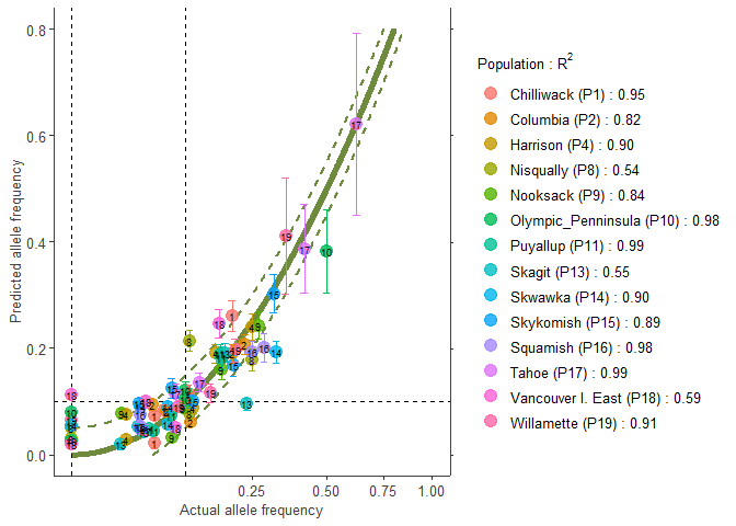
# 4. Check how well the models predict baseline allele frequencies
# Populations are split in those with R2 > 0.50 and those with R2 < 0.50
# Better populations
plotA1 <- freq.ggplot(Poptri.freq.baseline,
plot.best=TRUE,
ylim=c(0.0, 0.8))
#> Pop Pop.label N GAM.rsq
#> 11 Puyallup 11 186 0.99
#> 17 Tahoe 17 12 0.99
#> 10 Olympic_Penninsula 10 5 0.98
#> 16 Squamish 16 14 0.98
#> 1 Chilliwack 1 38 0.95
#> 19 Willamette 19 17 0.91
#> 4 Harrison 4 22 0.90
#> 14 Skwawka 14 14 0.90
#> 15 Skykomish 15 156 0.89
#> 9 Nooksack 9 26 0.84
#> 2 Columbia 2 180 0.82
#> 18 Vancouver I. East 18 12 0.59
#> 13 Skagit 13 163 0.55
#> 8 Nisqually 8 14 0.54
#> 7 Klinaklini 7 8 0.42
#> 6 Kitimat 6 8 0.41
#> 12 Salmon 12 11 0.34
#> 5 Homathko 5 9 0.17
#> 3 Dean 3 7 0.15
#> [1] "Chilliwack" "Columbia" "Harrison"
#> [4] "Nisqually" "Nooksack" "Olympic_Penninsula"
#> [7] "Puyallup" "Skagit" "Skwawka"
#> [10] "Skykomish" "Squamish" "Tahoe"
#> [13] "Vancouver I. East" "Willamette"
plotA1
# Populations with low R2
manual.colour.values1 <- ggsci::pal_npg()(5)

plotB1 <- freq.ggplot(Poptri.freq.baseline,
            plot.best=FALSE,
            manual.colour.values=manual.colour.values1,
            xlim=c(0, 0.5),
            ylim=c(0, 0.25))
#>                   Pop Pop.label   N GAM.rsq
#> 11           Puyallup        11 186    0.99
#> 17              Tahoe        17  12    0.99
#> 10 Olympic_Penninsula        10   5    0.98
#> 16           Squamish        16  14    0.98
#> 1          Chilliwack         1  38    0.95
#> 19         Willamette        19  17    0.91
#> 4            Harrison         4  22    0.90
#> 14            Skwawka        14  14    0.90
#> 15          Skykomish        15 156    0.89
#> 9            Nooksack         9  26    0.84
#> 2            Columbia         2 180    0.82
#> 18  Vancouver I. East        18  12    0.59
#> 13             Skagit        13 163    0.55
#> 8           Nisqually         8  14    0.54
#> 7          Klinaklini         7   8    0.42
#> 6             Kitimat         6   8    0.41
#> 12             Salmon        12  11    0.34
#> 5            Homathko         5   9    0.17
#> 3                Dean         3   7    0.15
#> [1] "Dean"       "Homathko"   "Kitimat"    "Klinaklini" "Salmon"
plotB1
# Colouring by alleles

plotA2 <- freq.ggplot(Poptri.freq.baseline,
            colour.Pop=FALSE,
            plot.best=TRUE,
            ylim=c(0.0, 0.8),
            manual.colour.values=manual.colour.values1)
#>                   Pop Pop.label   N GAM.rsq
#> 11           Puyallup        11 186    0.99
#> 17              Tahoe        17  12    0.99
#> 10 Olympic_Penninsula        10   5    0.98
#> 16           Squamish        16  14    0.98
#> 1          Chilliwack         1  38    0.95
#> 19         Willamette        19  17    0.91
#> 4            Harrison         4  22    0.90
#> 14            Skwawka        14  14    0.90
#> 15          Skykomish        15 156    0.89
#> 9            Nooksack         9  26    0.84
#> 2            Columbia         2 180    0.82
#> 18  Vancouver I. East        18  12    0.59
#> 13             Skagit        13 163    0.55
#> 8           Nisqually         8  14    0.54
#> 7          Klinaklini         7   8    0.42
#> 6             Kitimat         6   8    0.41
#> 12             Salmon        12  11    0.34
#> 5            Homathko         5   9    0.17
#> 3                Dean         3   7    0.15
#>  [1] "Chilliwack"         "Columbia"           "Harrison"
#>  [4] "Nisqually"          "Nooksack"           "Olympic_Penninsula"
#>  [7] "Puyallup"           "Skagit"             "Skwawka"
#> [10] "Skykomish"          "Squamish"           "Tahoe"
#> [13] "Vancouver I. East"  "Willamette"

plotA2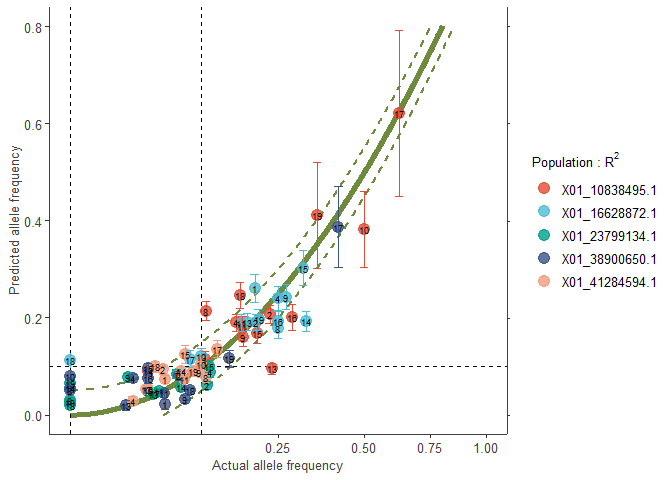
plotB2 <- freq.ggplot(Poptri.freq.baseline,
            colour.Pop=FALSE,
            plot.best=FALSE,
            manual.colour.values=manual.colour.values1,
            xlim=c(0, 0.5),
            ylim=c(0, 0.25))
#>                   Pop Pop.label   N GAM.rsq
#> 11           Puyallup        11 186    0.99
#> 17              Tahoe        17  12    0.99
#> 10 Olympic_Penninsula        10   5    0.98
#> 16           Squamish        16  14    0.98
#> 1          Chilliwack         1  38    0.95
#> 19         Willamette        19  17    0.91
#> 4            Harrison         4  22    0.90
#> 14            Skwawka        14  14    0.90
#> 15          Skykomish        15 156    0.89
#> 9            Nooksack         9  26    0.84
#> 2            Columbia         2 180    0.82
#> 18  Vancouver I. East        18  12    0.59
#> 13             Skagit        13 163    0.55
#> 8           Nisqually         8  14    0.54
#> 7          Klinaklini         7   8    0.42
#> 6             Kitimat         6   8    0.41
#> 12             Salmon        12  11    0.34
#> 5            Homathko         5   9    0.17
#> 3                Dean         3   7    0.15
#> [1] "Dean"       "Homathko"   "Kitimat"    "Klinaklini" "Salmon"

plotB2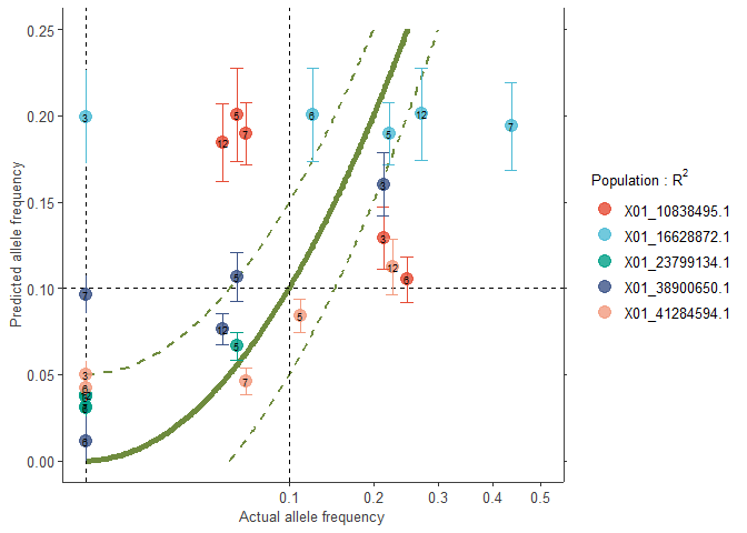
# Note that you can also compare data with:
poppr::poppr(Poptri.genind)
#>                   Pop   N MLG eMLG    SE     H    G lambda   E.5  Hexp       Ia
#> 1          Chilliwack  38  14 5.67 1.244 1.972 3.97  0.748 0.480 0.168  0.29948
#> 2            Columbia 180  31 6.69 1.276 2.634 8.17  0.878 0.555 0.219  0.03214
#> 3                Dean   7   4 4.00 0.000 1.352 3.77  0.735 0.967 0.145 -0.16667
#> 4            Harrison  22  10 5.87 1.093 1.855 4.10  0.756 0.575 0.191  0.06387
#> 5            Homathko   9   7 7.00 0.000 1.831 5.40  0.815 0.840 0.182 -0.17703
#> 6             Kitimat   8   4 4.00 0.000 1.321 3.56  0.719 0.930 0.127 -0.13245
#> 7          Klinaklini   8   5 5.00 0.000 1.494 4.00  0.750 0.868 0.155 -0.41248
#> 8           Nisqually  14   7 5.51 0.830 1.567 3.38  0.704 0.627 0.157  0.00845
#> 9            Nooksack  26  11 6.44 1.072 2.124 6.76  0.852 0.782 0.211  0.05709
#> 10 Olympic_Penninsula   5   3 3.00 0.000 0.950 2.27  0.560 0.802 0.191 -0.25000
#> 11           Puyallup 186  29 6.03 1.303 2.396 5.81  0.828 0.482 0.178 -0.02222
#> 12             Salmon  11   7 6.64 0.481 1.846 5.76  0.826 0.892 0.193 -0.19978
#> 13             Skagit 163  20 5.41 1.268 2.102 4.72  0.788 0.518 0.168 -0.01194
#> 14            Skwawka  14   6 5.29 0.656 1.631 4.45  0.776 0.841 0.160 -0.04804
#> 15          Skykomish 156  31 6.97 1.249 2.730 9.26  0.892 0.576 0.233  0.07931
#> 16           Squamish  14  10 7.86 0.802 2.206 8.17  0.878 0.887 0.205 -0.28884
#> 17              Tahoe  12   9 7.82 0.649 2.095 7.20  0.861 0.870 0.293 -0.11481
#> 18  Vancouver I. East  12   4 3.50 0.584 0.837 1.71  0.417 0.546 0.107  0.48361
#> 19         Willamette  17  10 6.65 1.016 2.007 5.45  0.817 0.691 0.246  0.11902
#> 20              Total 902  59 6.38 1.323 2.663 6.93  0.856 0.445 0.200  0.03621
#>       rbarD          File
#> 1   0.08166 Poptri.genind
#> 2   0.00883 Poptri.genind
#> 3  -0.16667 Poptri.genind
#> 4   0.02067 Poptri.genind
#> 5  -0.04770 Poptri.genind
#> 6  -0.14222 Poptri.genind
#> 7  -0.21444 Poptri.genind
#> 8   0.00445 Poptri.genind
#> 9   0.01646 Poptri.genind
#> 10 -0.25000 Poptri.genind
#> 11 -0.00606 Poptri.genind
#> 12 -0.07663 Poptri.genind
#> 13 -0.00373 Poptri.genind
#> 14 -0.01849 Poptri.genind
#> 15  0.02249 Poptri.genind
#> 16 -0.08273 Poptri.genind
#> 17 -0.03060 Poptri.genind
#> 18  0.27081 Poptri.genind
#> 19  0.04139 Poptri.genind
#> 20  0.00998 Poptri.genind
adegenet::makefreq(Poptri.genpop)
#>
#>  Finding allelic frequencies from a genpop object...
#>
#> ...done.
#>                    X01_10838495.1 X01_10838495.2 X01_16628872.1 X01_16628872.2
#> Chilliwack             0.10526316      0.8947368     0.19736842      0.8026316
#> Columbia               0.23055556      0.7694444     0.20000000      0.8000000
#> Dean                   0.21428571      0.7857143     0.00000000      1.0000000
#> Harrison               0.15909091      0.8409091     0.25000000      0.7500000
#> Homathko               0.05555556      0.9444444     0.22222222      0.7777778
#> Kitimat                0.25000000      0.7500000     0.12500000      0.8750000
#> Klinaklini             0.06250000      0.9375000     0.43750000      0.5625000
#> Nisqually              0.10714286      0.8928571     0.25000000      0.7500000
#> Nooksack               0.17307692      0.8269231     0.26923077      0.7307692
#> Olympic_Penninsula     0.50000000      0.5000000     0.10000000      0.9000000
#> Puyallup               0.17204301      0.8279570     0.16935484      0.8306452
#> Salmon                 0.04545455      0.9545455     0.27272727      0.7272727
#> Skagit                 0.23619632      0.7638037     0.18098160      0.8190184
#> Skwawka                0.03571429      0.9642857     0.32142857      0.6785714
#> Skykomish              0.20192308      0.7980769     0.31410256      0.6858974
#> Squamish               0.28571429      0.7142857     0.25000000      0.7500000
#> Tahoe                  0.62500000      0.3750000     0.08333333      0.9166667
#> Vancouver I. East      0.16666667      0.8333333     0.00000000      1.0000000
#> Willamette             0.35294118      0.6470588     0.20588235      0.7941176
#>                    X01_23799134.1 X01_23799134.2 X01_38900650.1 X01_38900650.2
#> Chilliwack             0.06578947      0.9342105     0.05263158      0.9473684
#> Columbia               0.10833333      0.8916667     0.06944444      0.9305556
#> Dean                   0.00000000      1.0000000     0.21428571      0.7857143
#> Harrison               0.11363636      0.8863636     0.02272727      0.9772727
#> Homathko               0.05555556      0.9444444     0.05555556      0.9444444
#> Kitimat                0.00000000      1.0000000     0.00000000      1.0000000
#> Klinaklini             0.00000000      1.0000000     0.00000000      1.0000000
#> Nisqually              0.00000000      1.0000000     0.00000000      1.0000000
#> Nooksack               0.01923077      0.9807692     0.07692308      0.9230769
#> Olympic_Penninsula     0.00000000      1.0000000     0.00000000      1.0000000
#> Puyallup               0.04569892      0.9543011     0.05107527      0.9489247
#> Salmon                 0.00000000      1.0000000     0.04545455      0.9545455
#> Skagit                 0.03987730      0.9601227     0.01840491      0.9815951
#> Skwawka                0.07142857      0.9285714     0.00000000      1.0000000
#> Skykomish              0.11217949      0.8878205     0.03525641      0.9647436
#> Squamish               0.03571429      0.9642857     0.03571429      0.9642857
#> Tahoe                  0.04166667      0.9583333     0.41666667      0.5833333
#> Vancouver I. East      0.00000000      1.0000000     0.08333333      0.9166667
#> Willamette             0.00000000      1.0000000     0.14705882      0.8529412
#>                    X01_41284594.1 X01_41284594.2
#> Chilliwack             0.05263158      0.9473684
#> Columbia               0.05000000      0.9500000
#> Dean                   0.00000000      1.0000000
#> Harrison               0.02272727      0.9772727
#> Homathko               0.11111111      0.8888889
#> Kitimat                0.00000000      1.0000000
#> Klinaklini             0.06250000      0.9375000
#> Nisqually              0.10714286      0.8928571
#> Nooksack               0.09615385      0.9038462
#> Olympic_Penninsula     0.10000000      0.9000000
#> Puyallup               0.07526882      0.9247312
#> Salmon                 0.22727273      0.7727273
#> Skagit                 0.03374233      0.9662577
#> Skwawka                0.07142857      0.9285714
#> Skykomish              0.07692308      0.9230769
#> Squamish               0.03571429      0.9642857
#> Tahoe                  0.12500000      0.8750000
#> Vancouver I. East      0.04166667      0.9583333
#> Willamette             0.08823529      0.9117647


# 5. Predict future allele frequencies

Poptri.pred.future <- count.pred(Poptri.count.model, env.data=future.env)
head(Poptri.pred.future)
#>           Pop Pop.label Pop.index   N         Allele Allele.freq  A   B
#> P1 Chilliwack         1         1  76 X01_10838495.1  0.10526316  8  68
#> P2   Columbia         2         2 360 X01_10838495.1  0.23055556 83 277
#> P3       Dean         3         3  14 X01_10838495.1  0.21428571  3  11
#> P4   Harrison         4         4  44 X01_10838495.1  0.15909091  7  37
#> P5   Homathko         5         5  18 X01_10838495.1  0.05555556  1  17
#> P6    Kitimat         6         6  16 X01_10838495.1  0.25000000  4  12
#>            Ap        Bp N.e1   Freq.e1
#> P1  14.795377  61.20462   76 0.1946760
#> P2 180.233278 179.76672  360 0.5006480
#> P3   2.158522  11.84148   14 0.1541801
#> P4  14.307597  29.69240   44 0.3251727
#> P5   4.778511  13.22149   18 0.2654728
#> P6   1.939753  14.06025   16 0.1212346

Poptri.freq.future <- freq.pred(Poptri.freq.model,
                                count.predicted=Poptri.pred.future)

# The key results are variables 'Allele.freq' representing the baseline allele frequencies
# and variables 'Freq.e2', the predicted frequency for the future/ past climate.
# Variable 'Freq.e1' is the predicted allele frequency in step 1

head(Poptri.freq.future)
#>           Pop Pop.label Pop.index   N         Allele Allele.freq  A   B
#> P1 Chilliwack         1         1  76 X01_10838495.1  0.10526316  8  68
#> P2   Columbia         2         2 360 X01_10838495.1  0.23055556 83 277
#> P3       Dean         3         3  14 X01_10838495.1  0.21428571  3  11
#> P4   Harrison         4         4  44 X01_10838495.1  0.15909091  7  37
#> P5   Homathko         5         5  18 X01_10838495.1  0.05555556  1  17
#> P6    Kitimat         6         6  16 X01_10838495.1  0.25000000  4  12
#>            Ap        Bp N.e1   Freq.e1   Freq.e2       LCL       UCL increasing
#> P1  14.795377  61.20462   76 0.1946760 0.1991648 0.1744943 0.2238354       TRUE
#> P2 180.233278 179.76672  360 0.5006480 0.5742628 0.4337850 0.7147405       TRUE
#> P3   2.158522  11.84148   14 0.1541801 0.1706418 0.1510378 0.1902458      FALSE
#> P4  14.307597  29.69240   44 0.3251727 0.3542175 0.3008643 0.4075707       TRUE
#> P5   4.778511  13.22149   18 0.2654728 0.2399923 0.2146111 0.2653735       TRUE
#> P6 1.939753 14.06025 16 0.1212346 0.1181220 0.1010202 0.1352239 FALSEdata(Poptri.baseline.env)
data(Poptri.future.env)
VIF.select <- VIF.subset(Poptri.baseline.env,
keep=c("MAT", "CMI"),
cor.plot=FALSE)
#> Step 1: Keeping these vars:
#> [1] "MAT" "CMI" "TD" "MSP" "AHM" "SHM" "DD.0" "bFFP"
#> [9] "PAS" "Eref" "CMD" "cmiJJA" "PPT_sm" "Tmax07"
#>
#> Variance inflation (package: car)
#> MAT TD MSP AHM SHM DD.0 bFFP
#> 1956.71402 55.35151 325.04715 258.27807 199.03579 383.71475 208.48116
#> PAS Eref CMD CMI cmiJJA PPT_sm Tmax07
#> 418.39278 509.80399 702.97284 729.58048 2108.47844 1221.60927 404.91923
#>
#> VIF directly calculated from linear model with focal numeric variable as response
#> cmiJJA MAT PPT_sm CMI CMD Eref PAS
#> 2108.47844 1956.71402 1221.60927 729.58048 702.97284 509.80399 418.39278
#> Tmax07 DD.0 MSP AHM bFFP SHM TD
#> 404.91923 383.71475 325.04715 258.27807 208.48116 199.03579 55.35151
#>
#> Variance inflation (package: car)
#> MAT TD MSP AHM SHM DD.0 bFFP
#> 1152.51188 51.00442 280.39905 196.06676 189.87780 289.82940 177.01912
#> PAS Eref CMD CMI PPT_sm Tmax07
#> 373.46930 302.59709 652.89020 548.59673 527.99218 186.61090
#>
#> VIF directly calculated from linear model with focal numeric variable as response
#> MAT CMD CMI PPT_sm PAS Eref DD.0
#> 1152.51188 652.89020 548.59673 527.99218 373.46930 302.59709 289.82940
#> MSP AHM SHM Tmax07 bFFP TD
#> 280.39905 196.06676 189.87780 186.61090 177.01912 51.00442
#>
#> Variance inflation (package: car)
#> MAT TD MSP AHM SHM DD.0 bFFP PAS
#> 775.21530 48.40917 275.40371 179.50626 90.11375 260.05137 146.29625 368.40367
#> Eref CMI PPT_sm Tmax07
#> 102.83305 545.11114 394.89879 180.19703
#>
#> VIF directly calculated from linear model with focal numeric variable as response
#> MAT CMI PPT_sm PAS MSP DD.0 Tmax07 AHM
#> 775.21530 545.11114 394.89879 368.40367 275.40371 260.05137 180.19703 179.50626
#> bFFP Eref SHM TD
#> 146.29625 102.83305 90.11375 48.40917
#>
#> Variance inflation (package: car)
#> MAT TD MSP AHM SHM DD.0 bFFP PAS
#> 528.61146 32.01349 145.93063 78.09567 53.38943 222.17330 145.00874 188.09374
#> Eref CMI Tmax07
#> 102.40225 306.50400 111.10074
#>
#> VIF directly calculated from linear model with focal numeric variable as response
#> MAT CMI DD.0 PAS MSP bFFP Tmax07 Eref
#> 528.61146 306.50400 222.17330 188.09374 145.93063 145.00874 111.10074 102.40225
#> AHM SHM TD
#> 78.09567 53.38943 32.01349
#>
#> Variance inflation (package: car)
#> MAT TD MSP AHM SHM bFFP PAS Eref
#> 291.46937 30.38197 64.59840 46.78232 37.94467 45.37584 45.57930 99.66232
#> CMI Tmax07
#> 93.58775 109.62229
#>
#> VIF directly calculated from linear model with focal numeric variable as response
#> MAT Tmax07 Eref CMI MSP AHM PAS bFFP
#> 291.46937 109.62229 99.66232 93.58775 64.59840 46.78232 45.57930 45.37584
#> SHM TD
#> 37.94467 30.38197
#>
#> Variance inflation (package: car)
#> MAT TD MSP AHM SHM bFFP PAS
#> 237.300281 4.513064 62.232526 46.486704 37.871152 44.616210 44.930713
#> Eref CMI
#> 33.411744 85.667431
#>
#> VIF directly calculated from linear model with focal numeric variable as response
#> MAT CMI MSP AHM PAS bFFP SHM
#> 237.300281 85.667431 62.232526 46.486704 44.930713 44.616210 37.871152
#> Eref TD
#> 33.411744 4.513064
#>
#> Variance inflation (package: car)
#> MAT TD AHM SHM bFFP PAS Eref
#> 218.240423 4.170754 25.872364 5.680412 43.733182 39.989330 32.625175
#> CMI
#> 27.162467
#>
#> VIF directly calculated from linear model with focal numeric variable as response
#> MAT bFFP PAS Eref CMI AHM SHM
#> 218.240423 43.733182 39.989330 32.625175 27.162467 25.872364 5.680412
#> TD
#> 4.170754
#>
#> Variance inflation (package: car)
#> MAT TD AHM SHM PAS Eref CMI
#> 56.168045 4.154401 24.524555 5.474406 31.877700 13.105090 22.368212
#>
#> VIF directly calculated from linear model with focal numeric variable as response
#> MAT PAS AHM CMI Eref SHM TD
#> 56.168045 31.877700 24.524555 22.368212 13.105090 5.474406 4.154401
#>
#> Variance inflation (package: car)
#> MAT TD AHM SHM Eref CMI
#> 8.713339 4.003336 19.299959 5.465614 9.025702 14.431931
#>
#> VIF directly calculated from linear model with focal numeric variable as response
#> AHM CMI Eref MAT SHM TD
#> 19.299959 14.431931 9.025702 8.713339 5.465614 4.003336
#>
#> Summary of VIF selection process:
#> MAT TD MSP AHM SHM DD.0 bFFP
#> step_1 1956.714025 55.351511 325.04715 258.27807 199.035789 383.7148 208.48116
#> step_2 1152.511883 51.004421 280.39905 196.06676 189.877801 289.8294 177.01912
#> step_3 775.215296 48.409171 275.40371 179.50626 90.113750 260.0514 146.29625
#> step_4 528.611459 32.013493 145.93063 78.09567 53.389431 222.1733 145.00874
#> step_5 291.469373 30.381965 64.59840 46.78232 37.944668 NA 45.37584
#> step_6 237.300281 4.513064 62.23253 46.48670 37.871152 NA 44.61621
#> step_7 218.240423 4.170754 NA 25.87236 5.680412 NA 43.73318
#> step_8 56.168045 4.154401 NA 24.52456 5.474406 NA NA
#> step_9 8.713339 4.003336 NA 19.29996 5.465614 NA NA
#> PAS Eref CMD CMI cmiJJA PPT_sm Tmax07
#> step_1 418.39278 509.803994 702.9728 729.58048 2108.478 1221.6093 404.9192
#> step_2 373.46930 302.597094 652.8902 548.59673 NA 527.9922 186.6109
#> step_3 368.40367 102.833047 NA 545.11114 NA 394.8988 180.1970
#> step_4 188.09374 102.402249 NA 306.50400 NA NA 111.1007
#> step_5 45.57930 99.662321 NA 93.58775 NA NA 109.6223
#> step_6 44.93071 33.411744 NA 85.66743 NA NA NA
#> step_7 39.98933 32.625175 NA 27.16247 NA NA NA
#> step_8 31.87770 13.105090 NA 22.36821 NA NA NA
#> step_9 NA 9.025702 NA 14.43193 NA NA NA
#>
#> Final selection of variables:
#> [1] "AHM" "CMI" "Eref" "MAT" "SHM" "TD"
VIF.select$vars.included
#> [1] "AHM" "CMI" "Eref" "MAT" "SHM" "TD"
baseline.env <- Poptri.baseline.env[, VIF.select$vars.included]
future.env <- Poptri.future.env[, VIF.select$vars.included]
plotA <- population.shift(baseline.env,
future.env,
option="PCA")
#> OK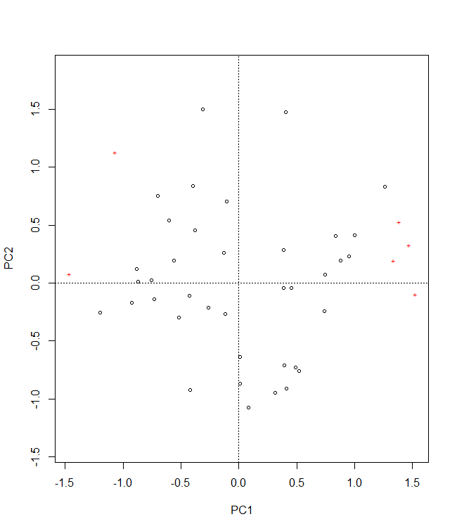
plotA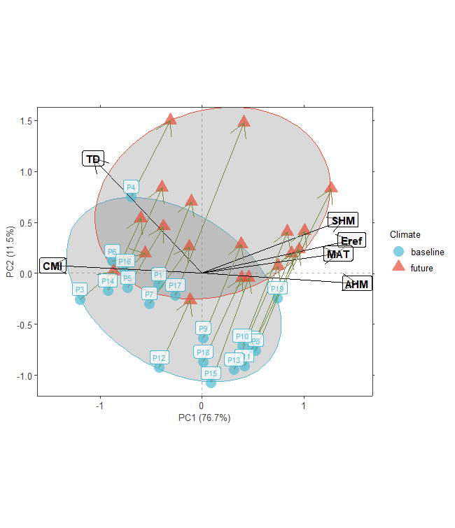
plotB <- population.shift(baseline.env,
                 future.env,
                 option="RDA")
#> OK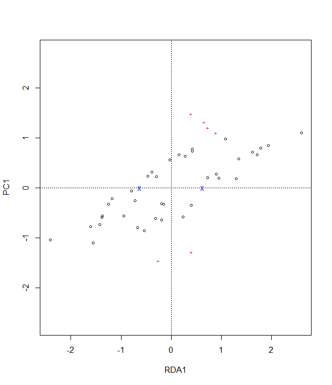
plotB
# The data can be obtained via the count.model and freq.model calibrations.
# These procedures are not repeated here.
data(Poptri.freq.future)

ggdot1 <- shift.dot.ggplot(Poptri.freq.future)
ggdot1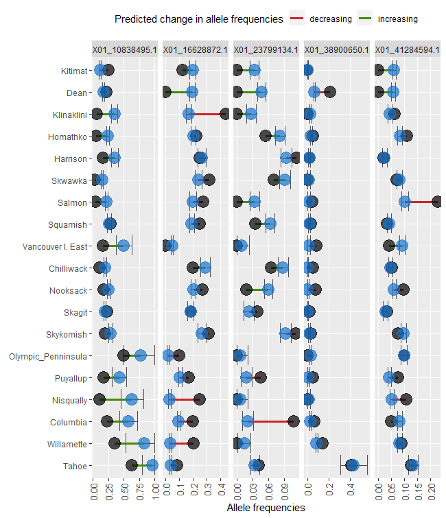
# The data can be obtained via the count.model and freq.model calibrations.
# These procedures are not repeated here.
data(Poptri.freq.baseline)
data(Poptri.freq.future)

Poptri.baseline.pie <- pie.baker(Poptri.freq.baseline, r0=0.1,
                                 sort.index="Latitude.index")

Poptri.future.pie <- pie.baker(Poptri.freq.future, r0=0.1,
                        freq.focus="Freq.e2",
                        sort.index="Latitude.index",
                        ypos=1)

ggpie1 <- shift.pie.ggplot(Poptri.baseline.pie,
                           Poptri.future.pie)
ggpie1
# The data can be obtained via the count.model and freq.model calibrations.
# These procedures are not repeated here.
data(Poptri.freq.baseline)
data(Poptri.freq.future)

Poptri.baseline.moon <- moon.waxer(Poptri.freq.baseline,
                                   sort.index="Latitude.index")

Poptri.future.moon <- moon.waxer(Poptri.freq.future,
                                 sort.index="Latitude.index",
                                 freq.focus="Freq.e2",
                                ypos=1)

ggmoon1 <- shift.moon.ggplot(Poptri.baseline.moon,
                             Poptri.future.moon)
ggmoon1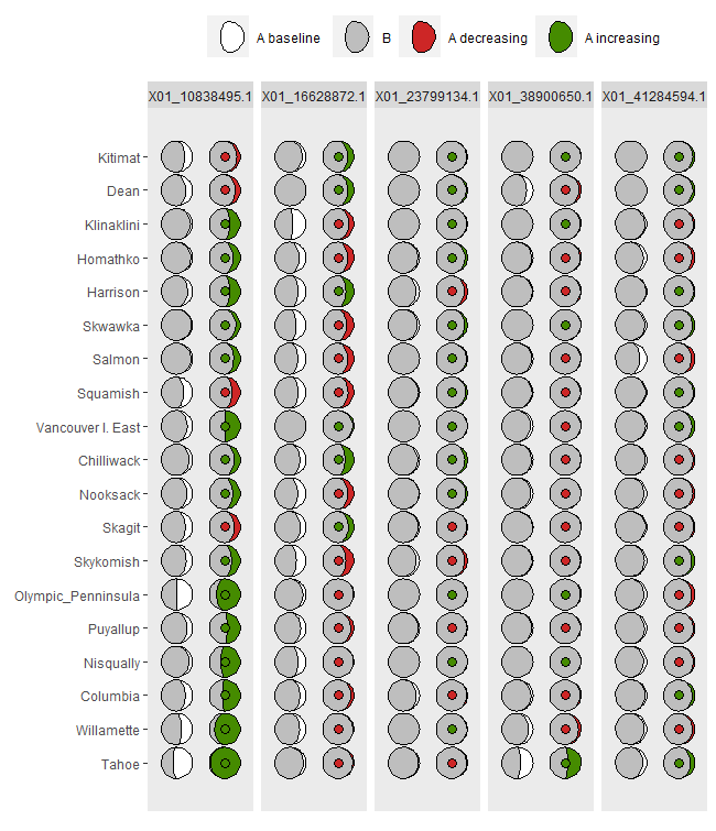
# The data can be obtained via the count.model and freq.model calibrations.
# These procedures are not repeated here.
data(Poptri.freq.baseline)
data(Poptri.freq.future)

Poptri.future.waffle <- waffle.baker(Poptri.freq.future,
                           sort.index="Latitude.index")

ggwaffle1 <- shift.waffle.ggplot(Poptri.future.waffle)
ggwaffle1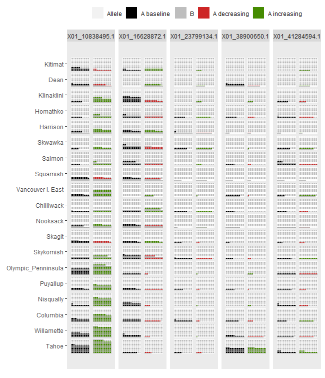
# The data can be obtained via the count.model and freq.model calibrations.
# These procedures are not repeated here.
data(Poptri.freq.baseline)
data(Poptri.freq.future)
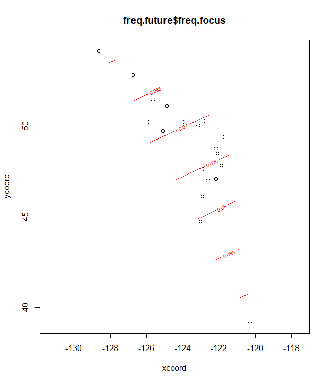
# Plots for the first allele
# Symbols and colours indicate future change (green, ^ = future increase)
# Symbol size reflects the frequency in the climate shown
# Baseline climate
plotA <- shift.surf.ggplot(Poptri.freq.future,
xcoord="Long", ycoord="Lat",
Allele.focus=unique(Poptri.freq.future$Allele)[1],
freq.focus="Allele.freq")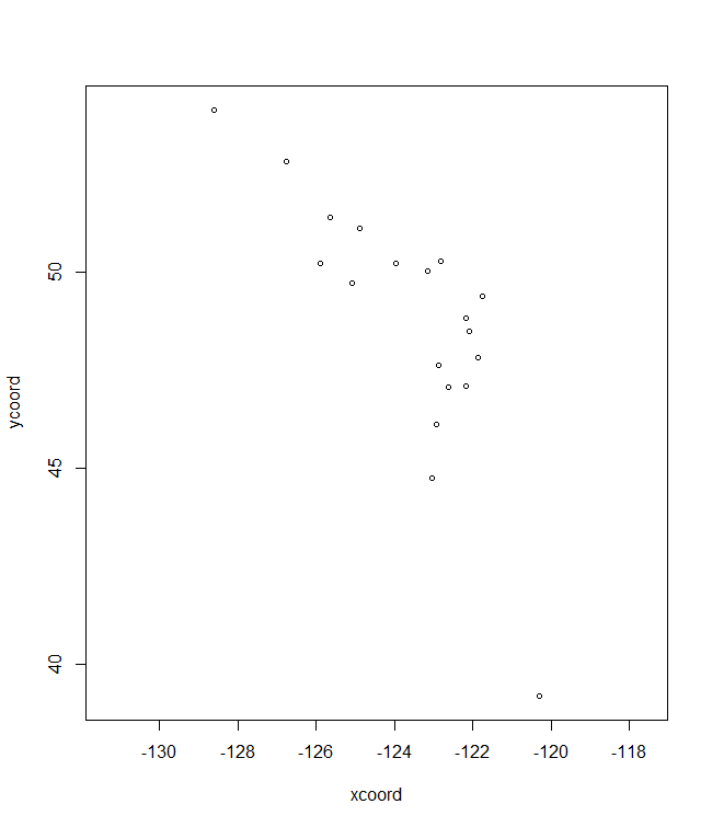
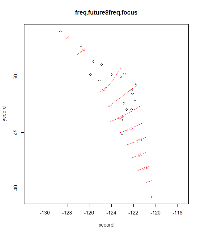
plotA
# Future/past climate
plotB <- shift.surf.ggplot(Poptri.freq.future,
                  xcoord="Long", ycoord="Lat",
                  Allele.focus=unique(Poptri.freq.future$Allele)[1],
                  freq.focus="Freq.e2")
plotB
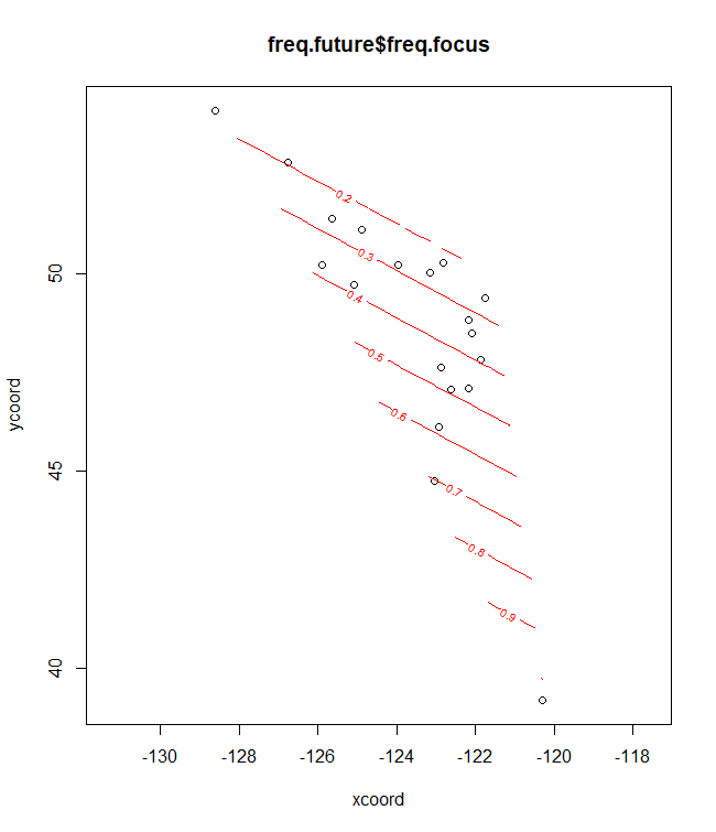
# Plots for the fifth allele

# Baseline climate
plotC <- shift.surf.ggplot(Poptri.freq.future,
                  xcoord="Long", ycoord="Lat",
                  Allele.focus=unique(Poptri.freq.future$Allele)[5],
                  freq.focus="Allele.freq")
plotC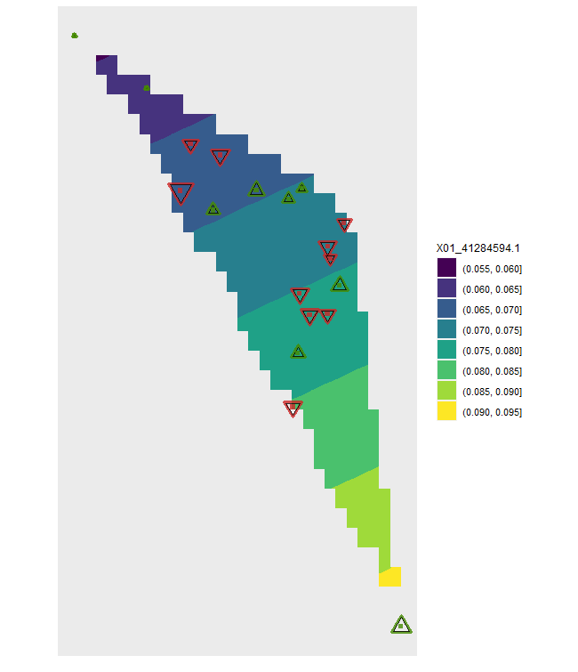
plotD <- shift.surf.ggplot(Poptri.freq.future,
                  xcoord="Long", ycoord="Lat",
                  Allele.focus=unique(Poptri.freq.future$Allele)[5],
                  freq.focus="Freq.e2")

plotD
With graphs that are generated via ggplot2, it is straightforward to create animations. The following example is also avaiable from the documentation of ‘AlleleShift::shift.dot.ggplot’
# create an animation

library(ggplot2)
library(gganimate)
library(gifski)
#> Warning: package 'gifski' was built under R version 4.0.3

# The data is an interpolation and extrapolation between the baseline and future climate.
# For actual application, interpolate between climate data from available sources

data(Poptri.1985to2085)

ggdot.all <- ggplot(data=Poptri.1985to2085, group=Decade) +
  scale_y_continuous(limits=c(-0.1, 1.1),
                     breaks=c(0.0, 0.25, 0.5, 0.75, 1.0)) +
  geom_errorbar(aes(x=Pop, ymin=LCL, ymax=UCL),
                colour="grey30", width=0.8, show.legend=FALSE) +
  geom_segment(aes(x=Pop, y=Allele.freq, xend=Pop, yend=Freq.e2, colour=increasing),
               size=1.2) +
  geom_point(aes(x=Pop, y=Allele.freq),
             colour="black", size=10, alpha=0.7) +
  geom_point(aes(x=Pop, y=Freq.e2),
             colour="dodgerblue3", size=10, alpha=0.7) +
  coord_flip() +
  xlab(element_blank()) +
  ylab("Allele frequencies") +
  theme(panel.grid.minor = element_blank()) +
  labs(colour="Future change in allele frequencies") +
  scale_colour_manual(values=c("firebrick3", "chartreuse4"),
                      labels=c("decreasing", "increasing")) +
  theme(axis.text.x=element_text(angle=90, vjust=0.5, size=10)) +
  theme(legend.position="top") +
  facet_grid( ~ Allele, scales="free")

ggdot.all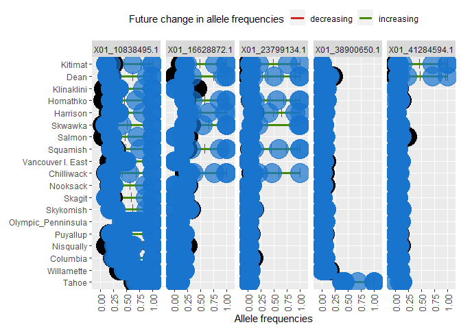
ggdot.anim <- ggdot.all +
  transition_states(as.factor(Decade), transition_length = 10, state_length = 100) +
  labs(title = "Decade: {closest_state}s")
Show the animation
animate(ggdot.anim, fps=5, width=1280, height=720)
sessionInfo()
#> R version 4.0.2 (2020-06-22)
#> Platform: x86_64-w64-mingw32/x64 (64-bit)
#> Running under: Windows 10 x64 (build 18363)
#>
#> Matrix products: default
#>
#> locale:
#> [1] LC_COLLATE=English_United Kingdom.1252
#> [2] LC_CTYPE=English_United Kingdom.1252
#> [3] LC_MONETARY=English_United Kingdom.1252
#> [4] LC_NUMERIC=C
#> [5] LC_TIME=English_United Kingdom.1252
#>
#> attached base packages:
#> [1] tcltk     stats     graphics  grDevices utils     datasets  methods
#> [8] base
#>
#> other attached packages:
#>  [1] gifski_0.8.6         AlleleShift_0.9      gganimate_1.0.7
#>  [4] gggibbous_0.1.0      ggmap_3.0.0          mgcv_1.8-31
#>  [7] nlme_3.1-148         GGally_2.0.0         patchwork_1.1.1
#> [10] ggrepel_0.8.2        dplyr_1.0.2          ggforce_0.3.2
#> [13] ggsci_2.9            ggplot2_3.3.2        poppr_2.8.6
#> [16] adegenet_2.1.3       ade4_1.7-16          BiodiversityR_2.12-3
#> [19] vegan_2.5-6          lattice_0.20-41      permute_0.9-5
#>
#> loaded via a namespace (and not attached):
#>   [1] readxl_1.3.1        backports_1.1.7     Hmisc_4.4-0
#>   [4] fastmatch_1.1-0     plyr_1.8.6          igraph_1.2.6
#>   [7] sp_1.4-2            splines_4.0.2       digest_0.6.25
#>  [10] htmltools_0.5.0     gdata_2.18.0        relimp_1.0-5
#>  [13] magrittr_1.5        checkmate_2.0.0     cluster_2.1.0
#>  [16] openxlsx_4.1.5      tcltk2_1.2-11       gmodels_2.18.1
#>  [19] sandwich_2.5-1      prettyunits_1.1.1   jpeg_0.1-8.1
#>  [22] colorspace_1.4-1    mitools_2.4         haven_2.3.1
#>  [25] xfun_0.15           crayon_1.3.4        lme4_1.1-23
#>  [28] survival_3.1-12     zoo_1.8-8           phangorn_2.5.5
#>  [31] ape_5.4             glue_1.4.1          polyclip_1.10-0
#>  [34] gtable_0.3.0        seqinr_4.2-4        polysat_1.7-4
#>  [37] car_3.0-8           abind_1.4-5         scales_1.1.1
#>  [40] DBI_1.1.0           Rcpp_1.0.4.6        isoband_0.2.1
#>  [43] viridisLite_0.3.0   xtable_1.8-4        progress_1.2.2
#>  [46] spData_0.3.8        htmlTable_2.0.0     units_0.6-7
#>  [49] foreign_0.8-80      spdep_1.1-5         Formula_1.2-3
#>  [52] survey_4.0          httr_1.4.2          htmlwidgets_1.5.1
#>  [55] RColorBrewer_1.1-2  acepack_1.4.1       ellipsis_0.3.1
#>  [58] reshape_0.8.8       pkgconfig_2.0.3     farver_2.0.3
#>  [61] nnet_7.3-14         deldir_0.2-3        labeling_0.3
#>  [64] tidyselect_1.1.0    rlang_0.4.8         reshape2_1.4.4
#>  [67] later_1.1.0.1       munsell_0.5.0       cellranger_1.1.0
#>  [70] tools_4.0.2         generics_0.1.0      evaluate_0.14
#>  [73] stringr_1.4.0       fastmap_1.0.1       yaml_2.2.1
#>  [76] knitr_1.28          zip_2.0.4           purrr_0.3.4
#>  [79] RgoogleMaps_1.4.5.3 mime_0.9            compiler_4.0.2
#>  [82] rstudioapi_0.11     curl_4.3            png_0.1-7
#>  [85] e1071_1.7-3         tibble_3.0.1        statmod_1.4.34
#>  [88] tweenr_1.0.1        stringi_1.4.6       forcats_0.5.0
#>  [91] Matrix_1.2-18       classInt_0.4-3      nloptr_1.2.2.1
#>  [94] vctrs_0.3.4         effects_4.1-4       RcmdrMisc_2.7-0
#>  [97] pillar_1.4.4        LearnBayes_2.15.1   lifecycle_0.2.0
#> [100] bitops_1.0-6        data.table_1.12.8   raster_3.4-5
#> [103] httpuv_1.5.4        R6_2.4.1            latticeExtra_0.6-29
#> [106] promises_1.1.1      KernSmooth_2.23-17  gridExtra_2.3
#> [109] rio_0.5.16          codetools_0.2-16    boot_1.3-25
#> [112] MASS_7.3-51.6       gtools_3.8.2        rjson_0.2.20
#> [115] withr_2.2.0         nortest_1.0-4       Rcmdr_2.6-2
#> [118] pegas_0.14          expm_0.999-5        parallel_4.0.2
#> [121] hms_0.5.3           quadprog_1.5-8      grid_4.0.2
#> [124] rpart_4.1-15        tidyr_1.1.2         coda_0.19-3
#> [127] class_7.3-17        minqa_1.2.4         rmarkdown_2.3
#> [130] carData_3.0-4       sf_0.9-6            shiny_1.4.0.2
#> [133] base64enc_0.1-3