CopSens implements the copula-based sensitivity analysis
method, as discussed in “Copula-based Sensitivity
Analysis for Multi-Treatment Causal Inference with Unobserved
Confounding”, with Gaussian copula adopted in particular.
You can install the development version from GitHub with:
# install.packages("devtools")
devtools::install_github("JiajingZ/CopSens")
The dependency pcaMethods from Bioconductor may fail to
automatically install, which would result in a warning similar to:
ERROR: dependency ‘pcaMethods’ is not available for package ‘CopSens’Then, please first install the pcaMethods manually
by
if (!requireNamespace("BiocManager", quietly = TRUE))
  install.packages("BiocManager")
BiocManager::install("pcaMethods")# load package #
library(CopSens)# load data #
y <- GaussianT_GaussianY$y
tr <- subset(GaussianT_GaussianY, select = -c(y))
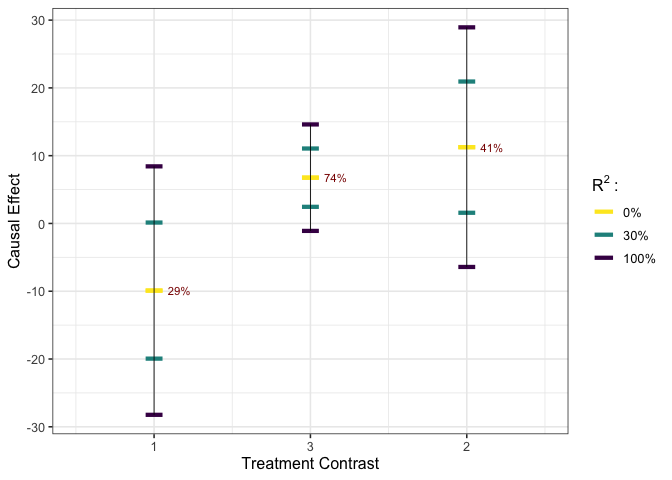
# execute worst-case calibration #
est_g1 <- gcalibrate(y = y, tr = tr, t1 = tr[c(1,2,1698),], tr[c(3,4,6698),],
calitype = "worstcase", R2 = c(0.3, 1))
#> Fitting the latent confounder model by PPCA with default.
#> 1:2:3:4:5:6:7:8:9:10:1:2:3:4:5:6:7:8:9:10:1:2:3:4:5:6:7:8:9:10:1:2:3:4:5:6:7:8:9:10:1:2:3:4:5:6:7:8:9:10:
#> Observed outcome model fitted by simple linear regression with default.
#> Worst-case calibration executed.
# visualize #
plot_estimates(est_g1, show_rv = TRUE)
# execute multivariate calibration #
est_g2 <- gcalibrate(y = y, tr = tr, t1 = tr[1:10,], t2 = tr[11:20,],
                     calitype = "multicali", R2_constr = c(1, 0.15))
#> Fitting the latent confounder model by PPCA with default.
#> 1:2:3:4:5:6:7:8:9:10:1:2:3:4:5:6:7:8:9:10:1:2:3:4:5:6:7:8:9:10:1:2:3:4:5:6:7:8:9:10:1:2:3:4:5:6:7:8:9:10:
#> Observed outcome model fitted by simple linear regression with default.
#> Multivariate calibration executed.
#> Calibrating with R2_constr =
#> 1
#> 0.15
#>
# visualize #
plot_estimates(est_g2)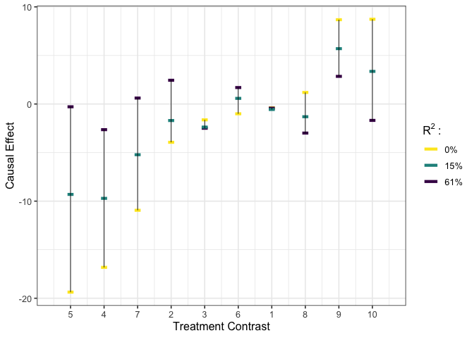
# execute user-specified calibration #
est_g3 <- gcalibrate(y = y, tr = tr, t1 = tr[1:2,], t2 = tr[3:4,],
                     calitype = "null", gamma = c(0.96, -0.29, 0),
                     R2 = c(0.2, 0.6, 1))
#> Fitting the latent confounder model by PPCA with default.
#> 1:2:3:4:5:6:7:8:9:10:1:2:3:4:5:6:7:8:9:10:1:2:3:4:5:6:7:8:9:10:1:2:3:4:5:6:7:8:9:10:1:2:3:4:5:6:7:8:9:10:
#> Observed outcome model fitted by simple linear regression with default.
#> User-specified calibration executed.
#>
# visualize #
plot_estimates(est_g3)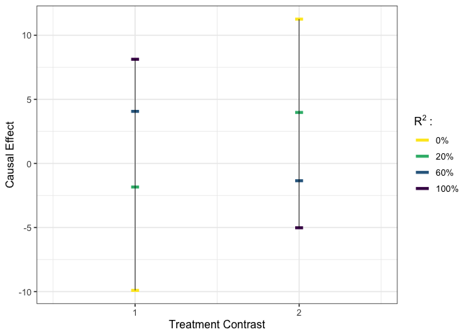
# apply gamma that maximizes the bias for the first contrast considered in est_g1 #
est_g4 <- gcalibrate(y = y, tr = tr, t1 = tr[1:2,], t2 = tr[3:4,],
                     calitype = "null", gamma = est_g1$gamma[1,],
                     R2 = c(0.2, 0.6, 1))
#> Fitting the latent confounder model by PPCA with default.
#> 1:2:3:4:5:6:7:8:9:10:1:2:3:4:5:6:7:8:9:10:1:2:3:4:5:6:7:8:9:10:1:2:3:4:5:6:7:8:9:10:1:2:3:4:5:6:7:8:9:10:
#> Observed outcome model fitted by simple linear regression with default.
#> User-specified calibration executed.
#>
# visualize #
plot_estimates(est_g4)
# load data #
y <- GaussianT_BinaryY$y
tr <- subset(GaussianT_BinaryY, select = -c(y))
t1 <- tr[1:5,]
t2 <- rep(0, times = ncol(tr))

# calibrate #
est_b <- bcalibrate(y = y, tr = tr, t = rbind(t1, t2),
                    gamma = c(1.27, -0.28, 0),
                    R2 = c(0.2, 0.7))
#> Fitting the latent confounder model by PPCA with default.
#> 1:2:3:4:5:6:7:8:9:10:1:2:3:4:5:6:7:8:9:10:1:2:3:4:5:6:7:8:9:10:1:2:3:4:5:6:7:8:9:10:1:2:3:4:5:6:7:8:9:10:
#> Observed outcome model fitted by simple probit model with default.
#> R2 = 0.2, calibrating observation
#> 1
#> 2
#> 3
#> 4
#> 5
#> 6
#>
#> R2 = 0.7, calibrating observation
#> 1
#> 2
#> 3
#> 4
#> 5
#> 6
#>
# calculate risk ratio estimator #
est_b_rr <- list(est_df = est_b$est_df[1:5,] / as.numeric(est_b$est_df[6,]),
                 R2 = c(0.2, 0.7))
# visualize #
plot_estimates(est_b_rr)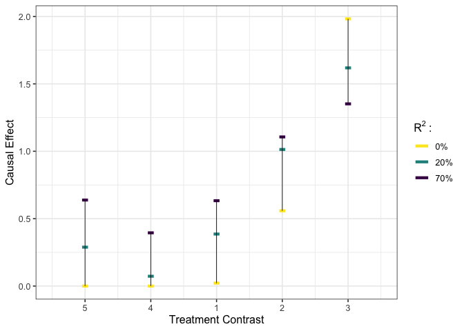
For further illustration, we compare our approach to a recent analysis of a mouse obesity dataset (Wang et al. (2006)), conducted by Miao et al. (2020), where the effect of gene expressions on the body weight of F2 mice is of interest. The data are collected from 287 mice, including the body weight, 37 gene expressions, and 5 single nucleotide polymorphisms. Among these 37 genes, 17 are likely to affect mouse weight (Lin et al. (2015)). In our example here, we focus on estimating the treatment effects of these 17 genes, and consider the comparison to the null treatments approach from Miao et al. (2020), which assumes that at least half of the confounded treatments have no causal effect on the outcome.
# load the data #
y <- micedata[,1]
tr <- micedata[, 2:18]
Following Miao et al. (2020), we infer a Gaussian conditional confounder distribution by applying factor analysis to treatments, and fit the observed outcome distribution with a linear regression.
# treatment model #
nfact <- 1
tr_factanal <- factanal(tr, factors=nfact, scores = "regression")
B_hat <- diag(sqrt(diag(var(tr)))) %*% tr_factanal$loadings
Sigma_t_u_hat <- diag(tr_factanal$uniquenesses * sqrt(diag(var(tr))))
u_hat <- tr_factanal$scores
coef_mu_u_t_hat <- t(B_hat) %*% solve(B_hat %*% t(B_hat) + Sigma_t_u_hat)
cov_u_t_hat <- diag(nfact) - t(B_hat) %*% solve(B_hat %*% t(B_hat) + Sigma_t_u_hat) %*% B_hat

# outcome model #
lmfit_y_t <- lm(y ~ ., data = micedata[,1:18])
beta_t <- coef(lmfit_y_t)[-1]
names(beta_t) <- colnames(tr)
sigma_y_t_hat <- sigma(lmfit_y_t)
We explore the ignorance regions for each treatment as well as causal estimates with multiple contrast criteria (MCCs) using the method described in Zheng, D’Amour and Franks (2021).
k <- ncol(tr)
t1 <- diag(k)
t2 <- matrix(0, ncol = k, nrow = k)
u_t_diff <- (t1 - t2) %*% t(coef_mu_u_t_hat)

# worst-case calibration #
R2 <- c(0.15, 0.5, 1)
worstcase_results <- gcalibrate(y, tr, t1 = t1, t2 = t2, calitype = "worstcase",
                                  mu_y_dt = as.matrix(beta_t), sigma_y_t =  sigma_y_t_hat,
                                  mu_u_dt = u_t_diff, cov_u_t = cov_u_t_hat, R2 = R2)
#> Worst-case calibration executed.
rownames(worstcase_results$est_df) <- names(beta_t)
names(worstcase_results$rv) <- names(beta_t)
plot_estimates(worstcase_results, order = "worstcase", labels = names(beta_t),
               axis.text.x = element_text(size = 10, angle = 75, hjust = 1))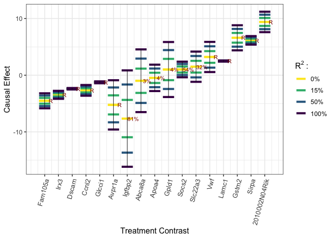
## multivariate calibration ##
# with L1 norm #
multcali_results_L1 <- gcalibrate(y, tr, t1 = t1, t2 = t2, calitype = "multicali",
mu_y_dt = as.matrix(beta_t), sigma_y_t = sigma_y_t_hat,
mu_u_dt = u_t_diff, cov_u_t = cov_u_t_hat, normtype = "L1")
#> Multivariate calibration executed.
#> Calibrating with R2_constr =
#> 1
#>
# with L2 norm #
multcali_results_L2 <- gcalibrate(y, tr, t1 = t1, t2 = t2, calitype = "multicali",
mu_y_dt = as.matrix(beta_t), sigma_y_t = sigma_y_t_hat,
mu_u_dt = u_t_diff, cov_u_t = cov_u_t_hat, normtype = "L2")
#> Multivariate calibration executed.
#> Calibrating with R2_constr =
#> 1
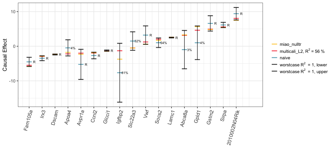
#> Below, we visualize the analysis results. The Spearman’s rank correlation between the estimated treatment effects of Miao et al. (2020) with the null treatment assumption (“miao_nulltr”) and ones by our MCC procedure with the L1 (“multicali_L1”) or L2 minimization (“multicali_L2”) is 0.90 or 0.93 respectively. In the plot below, the blue, green and yellow bars are closely grouped together for majority of treatments.
order_name <- rownames(multcali_results_L2$est_df)[order(multcali_results_L2$est_df[,2])]
summary_df <- data.frame(uncali = round(multcali_results_L2$est_df[order_name, 1], 3),
                         multicali_L1 = round(multcali_results_L1$est_df[order_name, 2], 3),
                         multicali_L2 = round(multcali_results_L2$est_df[order_name, 2], 3),
                         miao_nulltr =  mice_est_nulltr[order_name,]$esti,
                         miao_nulltr_sig = mice_est_nulltr[order_name,]$signif,
                         worstcase_lwr = worstcase_results$est_df[order_name, 'R2_1_lwr'],
                         worstcase_upr = worstcase_results$est_df[order_name, 'R2_1_upr'])
rownames(summary_df) <- order_name
plot_L1L2Null <- data.frame(summary_df[,c(1:4)], case = 1:nrow(summary_df)) %>%
  gather(key = "Type", value = "effect", - case) %>%
  ggplot() +
  ungeviz::geom_hpline(aes(x = case, y = effect, col = Type), width = 0.5, size = 1.2)  +
  scale_colour_manual(name = "",
                      values = c("#3B99B1", "#7CBA96", "#FFC300", "#F5191C"),
                      # divergingx_hcl(5, palette = "Zissou 1")[c(1, 2, 3, 5)],
                      labels = c("miao_nulltr",
                                 bquote("multicali_L1,"~R^2~"="~
                                              .(round(multcali_results_L1$R2*100,0))~"%"),
                                 bquote("multicali_L2,"~R^2~"="~
                                              .(round(multcali_results_L2$R2*100,0))~"%"),
                                 "naive")) +
  scale_x_continuous(breaks = 1:k, labels = order_name,
                     limits = c(0.5,k + 0.5)) +
  labs(y = "Causal Effect", x = "") +
  theme_bw(base_size = 14) +
  theme(plot.title = element_text(hjust = 0.5),
        axis.text.x = element_text(size = 13, angle = 75, hjust = 1),
        legend.text.align = 0,
        legend.title = element_text(size=10))
print(plot_L1L2Null)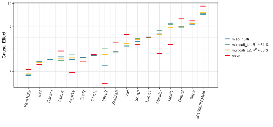
We also explore the worst-case ignorance region for each treatment under the Gaussian copula assumption. Even though, this assumption may not hold in practice, we can still see in the plot that 16/17 of Miao et al. (2020)’s causal estimates with null treatment assumption (“miao_nulltr”) are covered by our ignorance region (“worstcase R2 = 1, lower”; “worstcase R2 = 1, upper”). The only exception, “2010002N04Rik”, whose causal effects by Miao et al. (2020) is, nevertheless, quite close to the lower bound.
bound_df <- tibble(x1 = 1:nrow(summary_df),
                 y1 = summary_df$worstcase_lwr,
                 x2 = 1:nrow(summary_df),
                 y2 = summary_df$worstcase_upr)
rv_labels <- worstcase_results$rv
rv_labels[!is.na(worstcase_results$rv)] <- paste0(round(worstcase_results$rv[!is.na(worstcase_results$rv)]), "%")
rv_labels[is.na(worstcase_results$rv)] <- "R"
plot_L2NullWorst <-
  data.frame(summary_df[,c(1,3,4,6:7)], case = 1:nrow(summary_df)) %>%
    gather(key = "Type", value = "effect", - case) %>%
    ggplot() +
    ungeviz::geom_hpline(aes(x = case, y = effect, col = Type),
                         width = 0.4, size = 1, alpha = 0.8)  +
    geom_segment(data = bound_df, aes(x=x1, y=y1, xend=x2, yend=y2)) +
    scale_colour_manual(name = "",
                        values = c("#FFC300", "#F5191C", "#3B99B1", "black", "black"),
                        labels = c("miao_nulltr",
                                   bquote("multicali_L2,"~R^2~"="~
                                            .(round(multcali_results_L2$R2*100,0))~"%"),
                                   "naive",
                                   bquote("worstcase"~R^2~" = 1, lower"),
                                   bquote("worstcase"~R^2~" = 1, upper"))) +
    scale_x_continuous(breaks = (1:k), labels = order_name,
                       limits = c(1, k + 1.2)) +
    annotate(geom = "text", x = 1:nrow(summary_df) + 0.4, y = worstcase_results$est_df[order_name,'R2_0'],
                      size = 3, label = rv_labels[order_name]) +
    labs(y = "Causal Effect", x = "") +
    theme_bw(base_size = 14) +
    theme(plot.title = element_text(hjust = 0.5),
          axis.text.x = element_text(size = 13, angle = 75, hjust = 1),
          legend.text.align = 0,
          legend.title = element_text(size=10))
print(plot_L2NullWorst)