EcoEnsemble is an R package to set up, fit and sample from the ensemble framework described in Spence et al (2018) for time series outputs.
You can install the development version of EcoEnsemble using the
devtools package:
library(devtools)
install_github("CefasRepRes/EcoEnsemble")Fitting an ensemble model in EcoEnsemble is done in three main steps:
EnsemblePrior() constructor.fit_ensemble_model() function with simulator outputs,
observations and prior information. The ensemble model can be fit,
obtaining either the point estimate, which maximises the posterior
density, or running Markov chain Monte Carlo to generate a sample from
the posterior denisty of the ensemble model.generate_sample() function with the fitted ensemble object,
the discrepancy terms and the ensemble’s best guess of the truth can be
generated. Similarly to fit_ensemble_model(), this can
either be a point estimate or a full sample.We illustrate this process with datasets included with the package. EcoEnsemble comes loaded with the predicted biomasses of 4 species from 4 different mechanistic models of fish populations in the North Sea. It also includes statistical estimates of the biomasses from single-species stock assessments, and covariances for the model outputs and assessments. The models are run for different time periods and different species.
library(EcoEnsemble)
# Outputs from mizer. These are logs of the biomasses for each year in a simulation.
print(SSB_miz)| N.pout | Herring | Cod | Sole | |
|---|---|---|---|---|
| 1984 | 10.31706 | 13.33601 | 10.80006 | 10.98139 |
| 1985 | 12.07673 | 13.63592 | 10.46646 | 10.87285 |
| … | … | … | … | … |
| 2049 | 12.46354 | 14.02923 | 12.27473 | 10.80954 |
| 2050 | 12.46509 | 14.03027 | 12.27422 | 10.81003 |
To encode prior beliefs about how model discrepancies are related to
one another, use the EnsemblePrior() constructor. Default
values are available.
priors <- EnsemblePrior(4)or custom priors can be specified.
#Endoding prior beliefs. Details of the meanings of these terms can be found in the vignette or the documentation
num_species <- 4
priors <- EnsemblePrior(
  d = num_species,
  ind_st_params = IndSTPrior("lkj",  list(3, 2), 3, AR_params = c(1,1)),
  ind_lt_params = IndLTPrior(
    "beta",
    list(c(10,4,8, 7),c(2,3,1, 4)),
    list(matrix(5, num_species, num_species),
         matrix(0.5, num_species, num_species))
  ),
  sha_st_params = ShaSTPrior("inv_wishart",list(2, 1/3),list(5, diag(num_species))),
  sha_lt_params = 5,
  truth_params = TruthPrior(num_species, 10, list(3, 3), list(10, diag(num_species)))
)
This creates an EnsemblePrior object, which we can use
to fit the ensemble model using the fit_ensemble_model()
function and the data loaded with the package. When running a full MCMC
sampling of the posterior, this step may take some time. Samples can
then be generated from the resulting object using the
generate_sample() function.
fit <- fit_ensemble_model(observations = list(SSB_obs, Sigma_obs),
simulators = list(list(SSB_ewe, Sigma_ewe, "EwE"),
list(SSB_lm, Sigma_lm, "LeMans"),
list(SSB_miz, Sigma_miz, "mizer"),
list(SSB_fs, Sigma_fs, "FishSUMS")),
priors = priors)
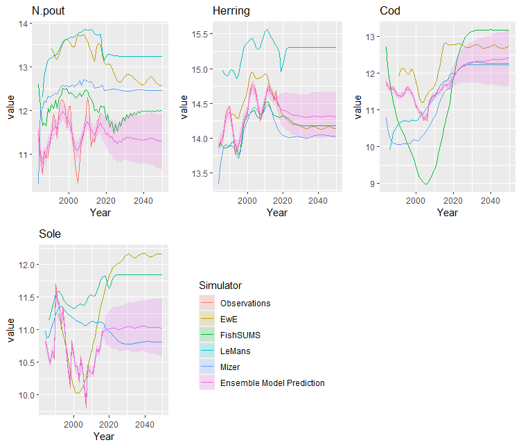
samples <- generate_sample(fit)This produces an EnsembleSample object containing
samples of the ensemble model predictions. These can be viewed by
calling the plot() function on this object. For a full MCMC
sample, this includes ribbons giving quantiles of the ensemble outputs.
If only maximising the posterior density, then only the single ouput is
plotted.
plot(samples)
Spence, M. A., J. L. Blanchard, A. G. Rossberg, M. R. Heath, J. J. Heymans, S. Mackinson, N. Serpetti, D. C. Speirs, R. B. Thorpe, and P. G. Blackwell. 2018. “A General Framework for Combining Ecosystem Models.” Fish and Fisheries 19: 1013–42.