![]()
Welcome to ICBioMark, based on the paper “Data-driven design of targeted gene panels for estimating immunotherapy biomarkers”, Bradley and Cannings (see our preprint).
You can install the release version of ICBioMark from CRAN with:
install.packages("ICBioMark")Alternatively, you can install the development version of this package from this github repository (using the devtools package) with:
devtools::install_github("cobrbra/ICBioMark")Upon installation we can load the package.
library(ICBioMark)To demonstrate the typical workflow for using ICBioMark, we play
around with a small and friendly example dataset. This is pre-loaded
with the package, but just comes from the data simulation function
generate_maf_data(), so you can play around with datasets
of different sizes and shapes.
Our example dataset, called example_maf_data, is a list
with two elements: maf and gene_lengths. These
are the two pieces of data that you’ll always need to use this package,
and they look as follows:
maf is a data frame in the MAF (mutation annotated
format) style. For a set of sequenced tumour/normal pairs, this means a
table with a row for every mutation identified, with columns
corresponding to properties such as the sample ID for the tumour of
origin, the gene, chromosome and nucelotide location of the mutation,
and the type of mutation observed. In the real world, MAF datasets often
have lots of extra information beyond this, but in our small example
we’ve just included sample, gene and mutation type (it’s all we’ll
need!). The top five rows look like this: # example_maf_data <- generate_maf_data()
kable(head(example_maf_data$maf, 5), row.names = FALSE)| Tumor_Sample_Barcode | Hugo_Symbol | Variant_Classification |
|---|---|---|
| SAMPLE_96 | GENE_14 | Missense_Mutation |
| SAMPLE_73 | GENE_14 | Frame_Shift_Ins |
| SAMPLE_55 | GENE_4 | Missense_Mutation |
| SAMPLE_96 | GENE_3 | Missense_Mutation |
| SAMPLE_38 | GENE_7 | Missense_Mutation |
gene_lengths, another data frame, this time containing
the names of genes that you’ll want to include in your modelling and
their length. Gene length is a complex and subtle thing to define - we
advise using coding length as defined in the Ensembl database. For this
example, however, gene lengths are again randomly chosen: kable(head(example_maf_data$gene_lengths, 5), row.names = FALSE)| Hugo_Symbol | max_cds |
|---|---|
| GENE_1 | 961 |
| GENE_2 | 1009 |
| GENE_3 | 1011 |
| GENE_4 | 976 |
| GENE_5 | 1016 |
These are the only two bits of data required to use ICBioMark. Your gene lengths data can contain values for far more genes than are observed in your dataset, and it’s not a huge problem if a couple of genes in a Whole-Exome Sequencing (WES) experiment are missing gene length information, but lots of missing values will cause issues with your model accuracy. Later versions of this package should be able to address missing gene length data.
The MAF format is widely used and standardised, but not especially
helpful for our purposes. The ideal format for our data is a matrix,
where every row corresponds to a sample, every column corresponds to a
gene/mutation type combination, and each entry corresponds to how many
mutations of that sample, gene and type were sequenced. At the same time
as this, we’d like to separate our training data from separately
reserved validation and test data. We do this using the function
get_mutation_tables().
Before we do this, however, we need to talk about mutation types. Our
procedure models different mutation types separately, so in theory one
could have separate parameters for each mutation type
(e.g. ‘Missense_Mutation’ or ‘Frame_Shift_Ins’). However, doing so will
vastly increase the computational complexity of fitting a generative
model. It is also not particularly informative to fit parameters to
extremely scarce mutation types. We therefore group mutation types
together (and can filter some out if we don’t want to include them in
our modelling). This will happen behind-the-scenes, but is worth knowing
about to understand the outputs generated. Mutations types are grouped
and filtered by the function get_mutation_dictionary(). In
general we recommend separately modelling indel mutations (so that we
can predict TIB later), synonymous mutations (as these don’t count
towards TMB or TIB), and lumping together all other nonsynonymous
mutation types. The function get_mutation_dictionary()
produces a list of mutation types, with labels for their groupings. For
example:
kable(get_mutation_dictionary(), col.names = "Label")| Label | |
|---|---|
| Missense_Mutation | NS |
| Nonsense_Mutation | NS |
| Splice_Site | NS |
| Translation_Start_Site | NS |
| Nonstop_Mutation | NS |
| In_Frame_Ins | NS |
| In_Frame_Del | NS |
| Frame_Shift_Del | I |
| Frame_Shift_Ins | I |
| Silent | S |
| Splice_Region | S |
| 3’Flank | S |
| 5’Flank | S |
| Intron | S |
| RNA | S |
| 3’UTR | S |
| 5’UTR | S |
We’ve given each mutation type one of three labels: “NS”, “S” and
“I”. We could have excluded synonymous mutation types by using
get_mutation_dictionary(include_synonymous = FALSE).
Now we can produce our training, validation and test sets (again for this example workflow these are pre-loaded). The object produced has three elements: ‘train’, ‘val’ and ‘test’. Each of these contains a sparse mutation matrix (‘matrix’) and other information describing the contents of the matrix (‘sample_list’, ‘gene_list’, ‘mut_types_list’ and ‘col_names’). We can see that the list of mutation types contains the three labels we specified above
  #example_tables <- get_mutation_tables(example_maf_data$maf,
  #                   sample_list = paste0("SAMPLE_", 1:100))

  print(example_tables$train$mut_types_list)
#> [1] "NS" "I"  "S"
and that the columns of each matrix correspond to each combination of mutation type and gene:
  print(head(example_tables$train$col_names, 10))
#>  [1] "GENE_1_NS" "GENE_1_I"  "GENE_1_S"  "GENE_2_NS" "GENE_2_I"  "GENE_2_S"
#> [7] "GENE_3_NS" "GENE_3_I" "GENE_3_S" "GENE_4_NS"There are relatively few decisions left to be made at this point: all
we need to do to fit a generative model is to provide gene lengths data
and training data to the function fit_gen_model(). We can
visualise output of our model with vis_model_fit().
  # example_gen_model <- fit_gen_model(example_maf_data$gene_lengths,
  #                       table = example_tables$train)

  print(vis_model_fit(example_gen_model))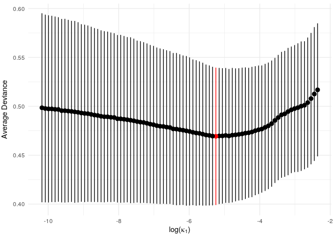
Since this is a small example, we don’t get a particularly strong
signal, but we do see an optimum level of penalisation. (NB: the
function vis_model_fit() essentially performs the same task
as glmnet::plot.cv.glmnet(). In later versions the
glmnet version will hopefully be directly applicable and
vis_model_fit() will be redundant).
We now construct a first-fit predictive model. The parameter
lambda controls the sparsity of each iteration, so it may
take some experimentation to get a good range of panel lengths.
  example_first_pred_tmb <- pred_first_fit(example_gen_model,
    lambda = exp(seq(-9, -14, length.out = 100)),
    training_matrix = example_tables$train$matrix,
    gene_lengths = example_maf_data$gene_lengths)
From this we can construct a range of refit estimators:
  example_refit_range <- pred_refit_range(pred_first = example_first_pred_tmb,
gene_lengths = example_maf_data$gene_lengths)With a predictive model fitted, we can use the function
get_predictions() along with a new (validation or test)
dataset to produce predictions on that dataset. We then provide several
functions including get_stats() to analyse the output
compared to true values.
  example_refit_range %>%
     get_predictions(new_data = example_tables$val) %>%
     get_stats(biomarker_values = example_tmb_tables$val, model = "T", threshold = 10) %>%
     ggplot(aes(x = panel_length, y = stat)) + geom_line() + facet_wrap(~metric) + theme_minimal() + labs(x = "Panel Length", y = "Predictive Performance")
Please do feel free to flag issues and requests on this repository. You can also email me.