LTASR

This package provides functions to replicate the CDC’s LTAS program within R. Currently, it will only stratify a cohort for fixed strata. It does not consider a history file for time-dependent exposures/variables.

It comes pre-installed with referent underlying cause of death (UCOD) rates for the 119 minors defined in Minors119 vignette for the US population.

Installation

You can install LTASR like so:

install.packages('LTASR')

Example

It is highly recommended to use R as well as RStudio. RStudio is a separate piece of software used to write and run R code.

It is highly recommended to use LTASR in conjunction with the tidyverse package. If this has not been installed yet, you will need to install it for your first use. Run:

install.packages('tidyverse')

This will only need to be run once, ever. It will install the necessary packages and functions to your computer.

The next step is to create a csv file containing the person level information. Each row of the file represents one unique person. The csv file must contain the following variables:

Variable	Description	Format
id	Unique identifier for each person
gender	Sex of person (“M” = male / “F” = female)	numeric
race	Race of person (“W” = white / “N” = nonwhite)	numeric
dob	date of birth	character
pybegin	date to begin follow-up	character
dlo	date last observed. Minimum of end of study, date of death, date lost to follow-up	character
vs	an indicator of ‘D’ for those who are deceased. All other values will be treated as alive or censored as of dlo.	character
code	ICD code of death; missing if person is censored or alive at study end date	character
rev	revision of ICD code (7-10); missing if person is censored or alive at study end date	numeric

Note: R variable names are case sensitive! All variable names must be lower case. This can be done in any software. Below is an example person file format:

id	gender	race	dob	pybegin	dlo	vs	rev	code
1	M	W	11/20/1945	12/21/1970	7/31/2016
2	M	N	3/15/1942	1/19/1972	8/19/2011	D	10	G30.9
3	F	W	6/5/1955	11/23/1970	12/7/1972	D	8	410.9

Once the person file has been created, there are several tools that can be used to read it into R. RStudio has a button in the top-right called ‘Import Dataset’ which provides tools for reading in data from various sources. This example will use the read_csv() function to read in the file into R (alternatively, other options are excel and SAS datasets from the ‘Import Dataset’ drop-down). The read_csv() function takes the file path of the person csv file as the first argument.

NOTE: Paths in R use forward slashes (/) instead of the standard back slashes () used by windows.

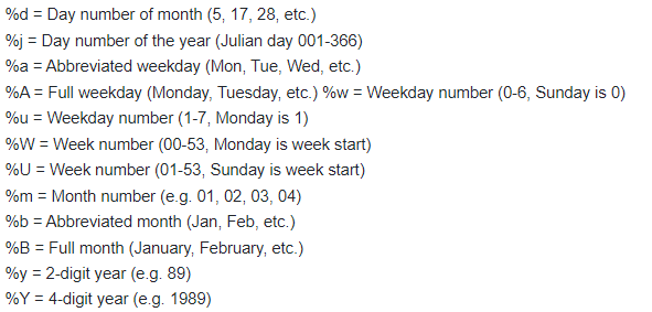
The date columns will need to be converted to R date values. This can be done using the as.Date() function. This function requires the user to specify the format of the dates being converted. Below gives a key in how to describe the date format:

So, the above date columns in the above example person file have the general format of “%m/%d/%Y”.
Below gives example code to read in the person file as well as code to convert the date columns to date values:

library(LTASR)
library(tidyverse)

person <- read_csv('C:/person.csv') %>%
  mutate(dob = as.Date(dob, format='%m/%d/%Y'),
         pybegin = as.Date(pybegin, format='%m/%d/%Y'),
         dlo = as.Date(dlo, format='%m/%d/%Y'))

The LTASR package comes with an example person file, called person_example, that can be used for testing. For this example, it will be read in, its dates will be converted and will be saved as ‘person’ similar to the above code:

person <- person_example %>%
  mutate(dob = as.Date(dob, format='%m/%d/%Y'),
         pybegin = as.Date(pybegin, format='%m/%d/%Y'),
         dlo = as.Date(dlo, format='%m/%d/%Y'))

Next, a rate file object must be created. This can be done using the parseRate() function and reading in an LTAS xml rate file. These xml files are available upon request and contain national population death rates for various outcomes. Below gives an example of reading in this file:

rateobj <- parseRate('C:/UCOD_WashingtonState012018.xml')

Alternatively, the LTASR package comes pre-installed with a rate object for the 119 LTAS minors of the US population from 1960-2020. This can be used in any analyses, but must be explicitly called first:

rateobj <- us_119ucod_19602020

Once a person file and a rate file have been read in, the get_table() function can be used to stratify the data from the person file according to the strata of the rate file (which is generally gender, race, 5-year age and 5-year calendar period categories):

py_table <- get_table(person, rateobj)

Once the py_table has been created, it can be saved using the write_csv() function. This file contains person day counts (pdays) and outcome counts for each minor (_o1, _o2, …..).
With your stratified data, you can quickly create a table with of all SMRs for each minor found in the rate file using the smr_minor() function as below:

smr_minor_table <- smr_minor(py_table, rateobj)

This table can be viewed with View() and saved with write_csv():

View(smr_minor_table)
write_csv(smr_minor_table, "C:/SMR_Minors.csv")

Next, SMRs for various groupings can be calculated from this table. One particular grouping are the Majors from LTAS found within the rate file. The smr_major() function can be used for this (reading in the smr_minor table created in the previous step):

smr_major_table <- smr_major(smr_minor_table, rateobj)
View(smr_major_table)
write_csv(smr_major_table, "C:/SMR_Majors")

Additionally, any custom grouping can be calculated as well using the smr_custom() function where grouping are defined as a vector of numbers. Below defines groupings for all deaths and all cancers:

minor_grouping <- 1:119
all_causes <- smr_custom(smr_minor_table, minor_grouping)
View(all_causes)

minor_grouping <- 4:40
all_cancers <- smr_custom(smr_minor_table, minor_grouping)
View(all_cancers)