The ‘QuantBondCurves’ package offers a range of functions for valuing various asset types and calibrating discount curves. It covers fixed-coupon assets, floating note assets and swaps, with varying payment frequencies. The package also enables the calibration of spot, instantaneous forward and basis curves, making it a powerful tool for accurate and flexible bond valuation and curve generation. The valuation and calibration techniques presented here are consistent with industry standards and incorporates author’s own calculations.
In light of the ongoing transition in the financial industry away from LIBOR, the inclusion of LIBOR in the package is intended to provide comprehensive coverage and enhance user convenience.
You can install QuantBondCurves from the CRAN repository with:
The ‘QuantBondCurves’ package offers the possibility of valuing various asset types. Below is a typical example for a bond indexed to 3M IBR rate.
# Calculates bond value
valuation.bonds(maturity = "2026-06-01", coupon.rate = 0.06, rates = 0.08, principal = 1000,
                analysis.date = "2025-06-01", asset.type = "IBR", freq = 4, rate.type = 1,
                daycount = "ACT/365")
#> [1] 983.1184
The process of valuing a bond can be broken down into multiple functions. In the following example, the various functions that comprise valuation.bonds are presented.
# Calculates coupon dates
coupon.dates(maturity = "2026-06-01", analysis.date = "2025-06-01",
             asset.type = "IBR")
#> $dates
#> [1] "2025-09-01" "2025-12-01" "2026-03-01" "2026-06-01"
#>
#> $effective.dates
#> [1] "2025-09-01" "2025-12-01" "2026-03-02" "2026-06-01"

# Calculates coupons
coupons(maturity = "2026-06-01" , analysis.date = "2025-06-01",
        coupon.rate = 0.06, principal = 1000, asset.type = "IBR")
#> [1]   15.33333   15.16667   15.00000 1015.33333

# Calculate discount factors
discount.factors(dates = c("2025-09-01", "2025-12-01", "2026-03-01", "2026-06-01"),
                 rates = c(0.01, 0.015, 0.017, 0.02), analysis.date = "2025-06-01",
                 rate.type = 1, freq = 4)
#> [1] 0.9974858 0.9925216 0.9873920 0.9802475
In addition to bond valuation, there are several other typical measures that can be calculated, such as the asset’s internal rate of return (IRR), accrued interest, bond sensitivity, or weighted average life. To illustrate these calculations, an example for each one is presented below:
# Calculates accrued interests
accrued.interests(maturity = '2026-06-01', analysis.date = "2025-06-01",
                  coupon.rate = 0.06, asset.type= 'IBR', daycount = "ACT/365")
#> [1] 0

# Calculate IRR of asset
bond.price2rate(maturity = "2026-06-01", price = 983.1184, analysis.date = "2025-06-01",
                coupon.rate = 0.06, principal = 1000, asset.type = "IBR", freq = 4,
                daycount = "ACT/365")
#> [1] 0.08000003

# Calculates bond sensitivity
sens.bonds(input = "price", price = 983.1184, maturity = "2026-06-01",
           analysis.date = "2025-06-01", coupon.rate = 0.06,
           principal = 1000, asset.type = "IBR", freq = 4,
           dirty = 1)
#> [1] 0.9055163

# Calculates weighted average life
average.life(input = c("rate"), price = 0.08, maturity = "2026-06-01",
             analysis.date = "2025-06-01", coupon.rate = 0.06,
             principal = 1000, asset.type = "IBR", freq = 4)
#> [1] 0.9778354
Lastly, with respect to valuation, the valuation.swaps function enables the process of valuing Interest Rate Swaps and Cross Currency Swaps. A straightforward example is offered for the former, as the latter may require basis curve calibration which can be accomplished using the calibration functions provided in the package.
# Calculates swap value
valuation.swaps(maturity = "2026-06-01", analysis.date = "2025-06-01",
coupon.rate = 0.02, rates = c(0.03,0.04,0.05,0.06),
float.rate = 0.03, principal = 1000)
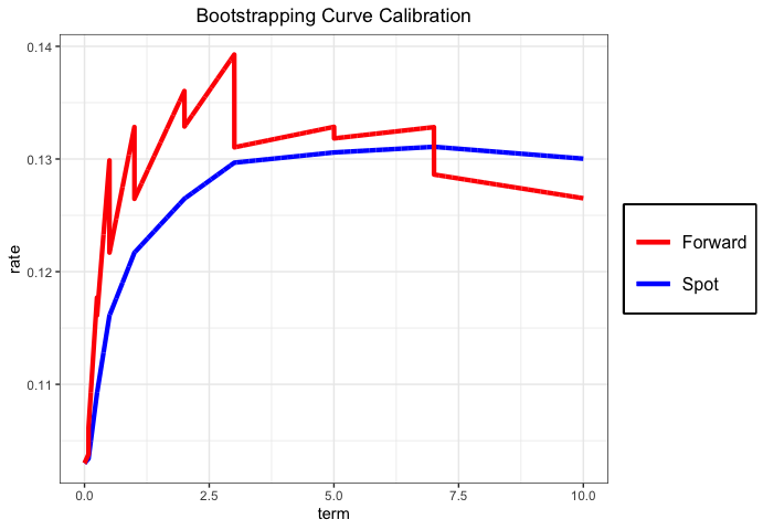
#> [1] 37.28375Another key feature of the package is curve calibration. These functions provide the capability to calibrate spot, forward, and basis curves in a flexible manner, allowing the user to choose over several methods for calibrating each curve. The package also allows for the transformation of spot to forward curves and vice versa. To demonstrate this feature, a simple example that outlines the process of spot calibration using the bootstrapping method is provided. Afterwards, output is transformed into a forward curve:
# Calibrates spot curve
yield.curve <- c(0.103,0.1034,0.1092, 0.1161, 0.1233, 0.1280, 0.1310, 0.1320,                   0.1325, 0.1320)
names(yield.curve) <- c(0,0.08,0.25,0.5,1,2,3,5,7,10)
nodes <- seq(0,10,0.001)

spot <- curve.calibration (yield.curve = yield.curve, market.assets = NULL,
                           analysis.date = "2019-01-03", asset.type = "IBRSwaps",
                           freq = 4, daycount = "ACT/365", fwd = 0, nodes = nodes,
                           approximation = "linear")

# Spot to forward
dates   <- names(spot)
forward <- spot2forward(dates, spot, approximation = "linear")
Below, the calibrated spot curve and its instantaneous forward equivalent are plotted: