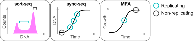
Repliscope is an R package for creating, normalising, comparing and plotting DNA replication timing profiles. The analysis pipeline starts with BED-formatted read count files (output of localMapper) obtained by high-throughput sequencing of DNA from replicating and non-replicating cells. There are three methods of measuring DNA replication dynamics using relative copy number (Fig): sort-seq, sync-seq and marker frequency analysis (MFA-seq). Sort-seq uses fluorescence-activated cell sorting (FACS) to enrich for non-replicating and replicating cells from an asynchronous population. Sync-seq requires cells to be arrested in non-replicating cell cycle phase (i.e. G1), followed by release into S phase. Samples are then taken throughout S phase when cells synchronously synthesise DNA according to the replication timing programme. In the case of MFA-seq, rapidly dividing cells in exponential growth phase are directly used as the replicating sample, while a saturated culture serves as a non-replicating control sample. While the latter approach of obtaining cells is the simplest, it also requires deeper sequencing due to decreased dynamic range and, thus, is more suitable for organisms with small genomes (typically, bacteria).
For best experience, use the Repliscope in interactive mode. To do so, simply run the runGUI() function.
The typical command line analysis using Repliscope starts with
loading BED-formatted read count files using the loadBed
function. Various functions allow removal of genomic bins containing low
quality data (rmChr,rmOutliers). To aid read
count analysis, two visualisation functions are used:
plotBed and plotCoverage. Next, read-depth
adjusted ratio of reads from the replicating sample to reads in the
non-replicating sample is calculated using the makeRatio
function; the resulting ratio values are distributed around one. The
normaliseRatio function is then used to transpose the ratio
values to a biologically relevant relative DNA copy number scale
(typically, from 1 to 2). The normalised ratio values are, essentially,
replication timing profiles, where low values indicate late replication
and high values - early replication. The plotRatio function
helps to visualise the ratio values as a histogram. Genomic bins
containing unusually high or low ratio values may be removed using the
trimRatio function. smoothRatio uses cubic
spline to smooth replication profile data. compareRatios
can be used to calculate difference between two replication profiles
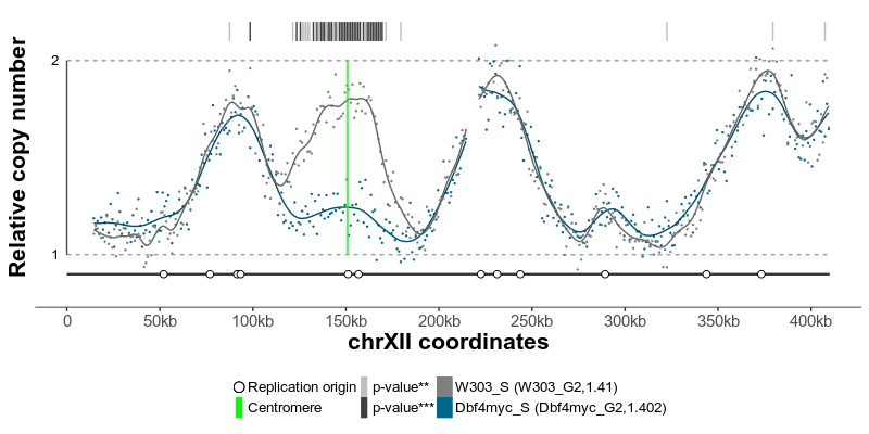
using z-score statistics. Finally, replication profiles are plotted
using the plotGenome function, which also allows for
various genome annotations.
You can install the released version of Repliscope from CRAN with:
install.packages("Repliscope")A typical analysis pipeline is below:
repBed <- loadBed('path/to/file1.bed')  # read counts from replicating sample
nrepRep <- loadBed('path/to/file2.bed')  # read counts from non-replicating sample
ratio <- makeRatio(repBed,nrepBed)  # create ratio between replicating and non-replicating samples
ratio <- normaliseRatio(ratio)  # normalise the ratio to fit biological scale of one to two
plotGenome(ratio) # plot the resulting replicating profileThe replication profiles may further be annotated with additional genomic data, such as location of centromeres, known replication origins or other regions or points of interest. Two replication profiles may be compared to find genomic regions with statistically different replication timing. Resulting plots may be saved as pdf files containing editable vector graphics.