An R package implementing the SE-set
algorithm, a tool to explore statistically-equivalent path
models from correlation matrices and Gaussian Graphical Models
(GGMs).
This repository contains an R package used by Ryan,
Bringmann and Schuurman (pre-print)[PsyArXiv] to aid researchers in
investigating the relationship between a given GGM estimate (in the form
of a precision matrix) and possible underlying linear path models.
Linear path models can also be interpreted as “weighted DAGs”. Full
details on the package can be found in Appendix B of
the manuscript, and code to reproduce the empirical illustration in that
paper can be found in this
repository.
Please note that we recommend the use of this tool only for GGMs with 13 or less nodes as the size of the outputted object, and the run-time, grows factorialy (\(p!\)) with each node in the network.
The current version of this package can be installed directly from github using
devtools::install_github("ryanoisin/SEset")The main SE-set function takes a precision matrix as input by default
(but can also take a matrix of partial correlations, or a covariance
matrix, detailed below). This can be estimated using packages such as
qgraph, using either raw data or a matrix of correlations.
For example, using the riskcor correlation matrix supplied
with the package as input, the precision matrix omega can
be estimated by running
# load data
data(riskcor)
# estimate precision matrix
estimate <- qgraph::EBICglasso(riskcor, n = 69, returnAllResults = TRUE)
omega <- estimate$optwi
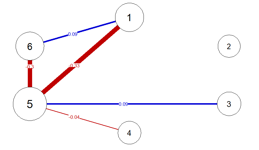
# The precision matrix can also be standardized to a partial correlation matrix, and plotted as a network
library(qgraph)
parcor <- qgraph::wi2net(omega)
pnet <- qgraph(parcor, repulsion = .8,vsize = c(10,15), theme = "colorblind", fade = F, edge.labels = TRUE)
Given a \(p\)-variate precision
matrix, the SEset package can be used to obtain a set of
maximally \(p!\) statistically
equivalent weighted DAGs (i.e., linear path models): One DAG for every
possible topological ordering of the \(p\) variables, from exogenous to
endogenous. This is the SE-set of omega which gives the
package its name.
The statistically-equivalent set is found by using the
network_to_SEset function
SE_example <- network_to_SEset(omega, digits = 2, rm_duplicates = TRUE)where the digits arguments determines the rounding of
parameters in the weighted DAGs, and the rm_duplicates
argument indicates that only unique weighted DAGs should be returned:
duplicates are removed after rounding. Typically, when duplicates are
removed, the number of unique DAGs returned is much less than \(p!\).
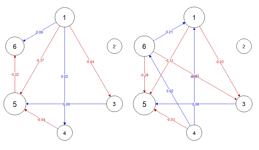
Individual members of the SE-set can be plotted, for example using
qgraph. When visualizing, remember that the weights matrix of the path
model \(B\) is given in SEM form \(X = BX +e\), and so should be read “from
column to row”, that is \(b_{ij}\)
encodes the direct effect of \(X_j\) on
\(X_i\). As a consequence, matrices
should be transposed when being used as input to qgraph and
most other network visualization tools.
DAG1 <- matrix(SE_example[1,],6,6)
DAG2 <- matrix(SE_example[30,],6,6)

par(mfrow=c(1,2))
qgraph(t(DAG1), repulsion = .8,vsize = c(10,15), theme = "colorblind", fade = F,
        layout = pnet$layout, maximum = 2, edge.labels = T)
qgraph(t(DAG2), repulsion = .8,vsize = c(10,15), theme = "colorblind", fade = F,
        layout = pnet$layout, maximum = 2, edge.labels = T)
We also supply additional functions to aid in exploring the SE-set.
For example, the function propcal calculates the
proportion of DAGs in the SE-set in which an edge between two variables
is present. You can choose distinguish between the presence of
some edge or an edge of a particular direction using the
directed option
# Undirected edge frequency
propu <- propcal(SE_example, rm_duplicate = F, directed = FALSE)

# Directed edge frequency
propd <- propcal(SE_example, rm_duplicate = F, directed = TRUE)

# Plot each as a network
par(mfrow=c(1,2))
qgraph(propu, edge.color = "darkgreen", layout = pnet$layout, edge.labels = T, maximum = 1)
qgraph(propd, edge.color = "darkgreen", layout = pnet$layout, edge.labels = T, maximum = 1)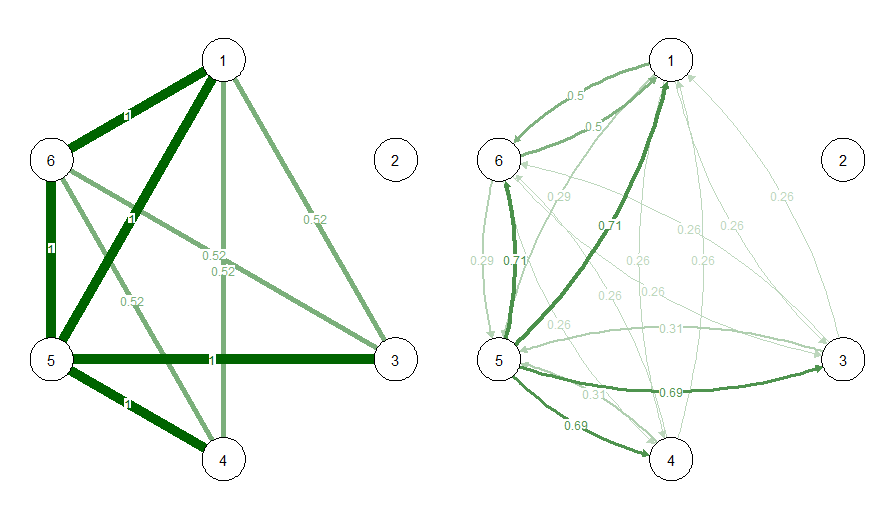
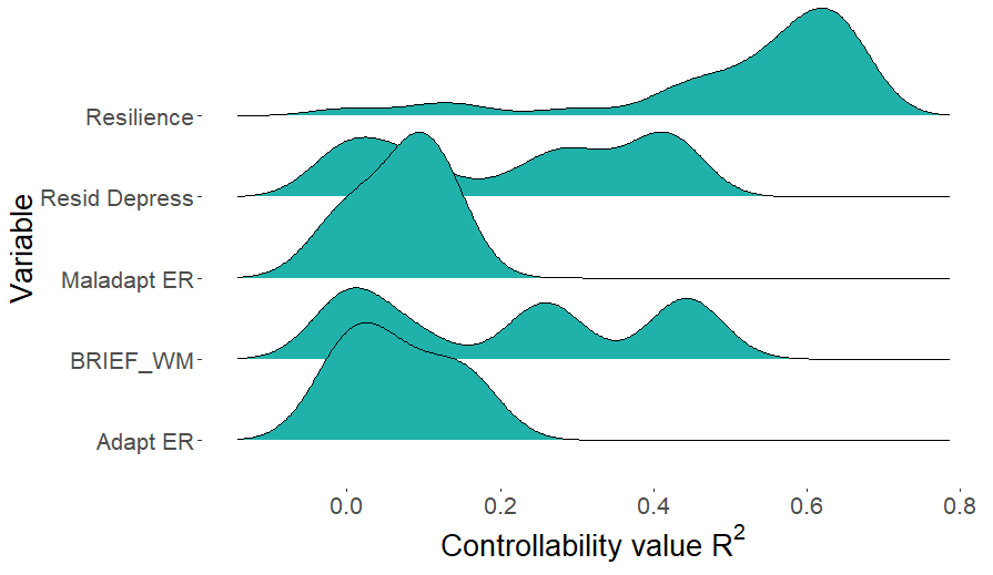
Given the SEset, you can essentially explore how any property of one
graphical model varies across members. For example, we may be interested
in the distribution of variance explained (\(R^2\)) for each variable when predicted by
it’s directed causes. This will differ across SEset members because the
direct casues of any given variable will typically differ across the
different path models. This can be computed using the
r2_distribution function.
r2set <- r2_distribution(SEmatrix = SE_example, cormat = riskcor, names = NULL,
                         indices = c(1,3,4,5,6))
This distribution can be visualized, for instance using ggplot
library(tidyr)
library(ggplot2)
require(ggridges)
df <- as.data.frame(r2set, col.names = paste0("X",1:6))

df2 <- tidyr::gather(df)

p <- ggplot(df2, aes(y = key, x = value)) +
  geom_density_ridges(fill = "light seagreen") +
  labs(y = "Variable", x = expression(paste("Controllability value ", R^2)))
p + theme(text = element_text(size = 20),
            axis.title.x = element_text(size = 20),
            axis.title.y = element_text(size = 20),
            panel.background = element_blank())
Alternatively, we can supply a matrix of partial
correlations, such as output by the parcor package, or
a (model-implied) covariance matrix using the
input_type argument, demonstrated below.
# Using the partial correlation matrix as input
SE_example_2 <- network_to_SEset(parcor, digits = 2, rm_duplicates = TRUE, input_type = "parcor")
# Calculating the model-implied covariance matrix from the precision matrix
MIcov <- solve(omega)
SE_example_3 <- network_to_SEset(MIcov, digits = 2, rm_duplicates = TRUE, input_type = "MIcov")
Note only that, since the partial correlation matrix does not contain
information on the diagonal elements of the precision matrix (that is,
the partial variances), if a partial correlation matrix is supplied, we
transform this to a correlation matrix using the corpcor
package. As such, small numerical differences (approximately in the 7th
decimal place) may be present depending on the input used.
For more details please contact o.ryan@uu.nl