The goal of SimMultiCorrData is to generate continuous
(normal or non-normal), binary, ordinal, and count (Poisson or Negative
Binomial) variables with a specified correlation matrix. It can also
produce a single continuous variable. This package can be used to
simulate data sets that mimic real-world situations (i.e. clinical data
sets, plasmodes, as in Vaughan et al., 2009). All variables are
generated from standard normal variables with an imposed intermediate
correlation matrix. Continuous variables are simulated by specifying
mean, variance, skewness, standardized kurtosis, and fifth and sixth
standardized cumulants using either Fleishman’s Third-Order or
Headrick’s Fifth-Order Polynomial Transformation. Binary and ordinal
variables are simulated using a modification of
GenOrd::ordsample. Count variables are simulated using the
inverse cdf method. There are two simulation pathways which differ
primarily according to the calculation of the intermediate correlation
matrix Sigma. In Correlation Method 1, the
intercorrelations involving count variables are determined using a
simulation based, logarithmic correlation correction (adapting Yahav and
Shmueli’s 2012 method). In Correlation Method 2, the
count variables are treated as ordinal (adapting Barbiero and Ferrari’s
2015 modification of GenOrd). There is an optional error
loop that corrects the final correlation matrix to be within a
user-specified precision value. The package also includes functions to
calculate standardized cumulants for theoretical distributions or from
real data sets, check if a target correlation matrix is within the
possible correlation bounds (given the distributions of the simulated
variables), summarize results (numerically or graphically), to verify
valid power method pdfs, and to calculate lower standardized kurtosis
bounds.
There are several vignettes which accompany this package that may help the user understand the simulation and analysis methods.
Benefits of SimMultiCorrData and Comparison to Other
Packages describes some of the ways
SimMultiCorrData improves upon other simulation
packages.
Variable Types describes the different types of
variables that can be simulated in
SimMultiCorrData.
Function by Topic describes each function, separated by topic.
Comparison of Correlation Method 1 and Correlation Method 2 describes the two simulation pathways that can be followed.
Overview of Error Loop details the algorithm involved in the optional error loop that improves the accuracy of the simulated variables’ correlation matrix.
Overall Workflow for Data Simulation gives a step-by-step guideline to follow with an example containing continuous (normal and non-normal), binary, ordinal, Poisson, and Negative Binomial variables. It also demonstrates the use of the standardized cumulant calculation function, correlation check functions, the lower kurtosis boundary function, and the plotting functions.
Comparison of Simulation Distribution to Theoretical Distribution or Empirical Data gives a step-by-step guideline for comparing a simulated univariate continuous distribution to the target distribution with an example.
Using the Sixth Cumulant Correction to Find Valid Power Method Pdfs demonstrates how to use the sixth cumulant correction to generate a valid power method pdf and the effects this has on the resulting distribution.
SimMultiCorrData can be installed using the following
code:
## from GitHub
install.packages("devtools")
devtools::install_github("AFialkowski/SimMultiCorrData")

## from CRAN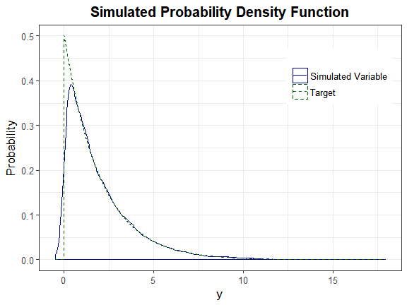
install.packages("SimMultiCorrData")This is a basic example which shows you how to solve a common problem: Compare a simulated exponential(mean = 2) variable to the theoretical exponential(mean = 2) density.
In R, the exponential parameter is rate <- 1/mean.
library(SimMultiCorrData)

stcums <- calc_theory(Dist = "Exponential", params = 0.5)
stcums
#>     mean       sd     skew kurtosis    fifth    sixth
#> 2 2 2 6 24 120Note that calc_theory returns the standard deviation,
not the variance. The simulation functions require variance as the
input.
H_exp <- nonnormvar1("Polynomial", means = stcums[1], vars = stcums[2]^2,
                     skews = stcums[3], skurts = stcums[4],
                     fifths = stcums[5], sixths = stcums[6], Six = NULL,
                     cstart = NULL, n = 10000, seed = 1234)
#> Constants: Distribution  1
#>
#> Constants calculation time: 0 minutes
#> Total Simulation time: 0.001 minutes

names(H_exp)
#> [1] "constants"           "continuous_variable" "summary_continuous"
#> [4] "summary_targetcont"  "sixth_correction"    "valid.pdf"
#> [7] "Constants_Time"      "Simulation_Time"
# Look at constants
H_exp$constants
#>           c0        c1       c2         c3          c4           c5
#> 1 -0.3077396 0.8005605 0.318764 0.03350012 -0.00367481 0.0001587077

# Look at summary
round(H_exp$summary_continuous[, c("Distribution", "mean", "sd", "skew",
                               "skurtosis", "fifth", "sixth")], 5)
#>    Distribution    mean     sd    skew skurtosis    fifth    sixth
#> X1 1 1.99987 2.0024 2.03382 6.18067 23.74145 100.3358H_exp$valid.pdf
#> [1] "TRUE"Let alpha = 0.05.
y_star <- qexp(1 - 0.05, rate = 0.5) # note that rate = 1/mean
y_star
#> [1] 5.991465Since the exponential(2) distribution has a mean and standard deviation equal to 2, solve \(\\Large 2 \* p(z') + 2 - y\_star = 0\) for \(\\Large z'\). Here, \(\\Large p(z') = c0 + c1 \* z' + c2 \* z'^2 + c3 \* z'^3 + c4 \* z'^4 + c5 \* z'^5\).
f_exp <- function(z, c, y) {
  return(2 * (c[1] + c[2] * z + c[3] * z^2 + c[4] * z^3 + c[5] * z^4 +
                c[6] * z^5) + 2 - y)
}

z_prime <- uniroot(f_exp, interval = c(-1e06, 1e06),
                   c = as.numeric(H_exp$constants), y = y_star)$root
z_prime
#> [1] 1.6449261 - pnorm(z_prime)
#> [1] 0.04999249This is approximately equal to the alpha value of 0.05, indicating the method provides a good approximation to the actual distribution.
plot_sim_pdf_theory(sim_y = as.numeric(H_exp$continuous_variable[, 1]),
                    overlay = TRUE, Dist = "Exponential", params = 0.5)
We can also plot the empirical cdf and show the cumulative probability up to y_star.
plot_sim_cdf(sim_y = as.numeric(H_exp$continuous_variable[, 1]),
             calc_cprob = TRUE, delta = y_star)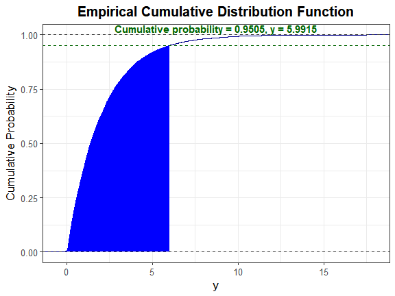
stats_pdf(c = H_exp$constants[1, ], method = "Polynomial", alpha = 0.025,
          mu = 2, sigma = 2)
#> trimmed_mean       median         mode   max_height
#>     1.858381     1.384521     0.104872     1.094213