

Cognostics are univariate statistics (or metrics) for a subset of
data. When paired with the underlying data of visualizations, cognostics
are a powerful tool for ordering and filtering the visualizations.
add_panel_cogs() will automatically append cognostics for
each plot player in a given panel column. The newly appended data can be
fed into a trelliscopejs widget
for easy viewing.
You can install autocogs from github with:
remotes::install_github("schloerke/autocogs")library(autocogs)
library(tidyverse)
#> ── Attaching packages ─────────────────────────────────────── tidyverse 1.3.0 ──
#> ✔ ggplot2 3.3.3.9000 ✔ purrr 0.3.4
#> ✔ tibble 3.1.1 ✔ dplyr 1.0.5
#> ✔ tidyr 1.1.3 ✔ stringr 1.4.0
#> ✔ readr 1.4.0 ✔ forcats 0.5.1
#> ── Conflicts ────────────────────────────────────────── tidyverse_conflicts() ──
#> ✖ dplyr::filter() masks stats::filter()
#> ✖ dplyr::lag() masks stats::lag()
library(gapminder)
# remotes::install_github("hafen/trelliscopejs")
# remotes::install_github("schloerke/trelliscopejs@autocogs")
library(trelliscopejs)
# Explore
p <-
ggplot(gapminder, aes(year, lifeExp)) +
geom_line(aes(group = country)) +
geom_smooth(method = "lm", formula = y ~ x)
p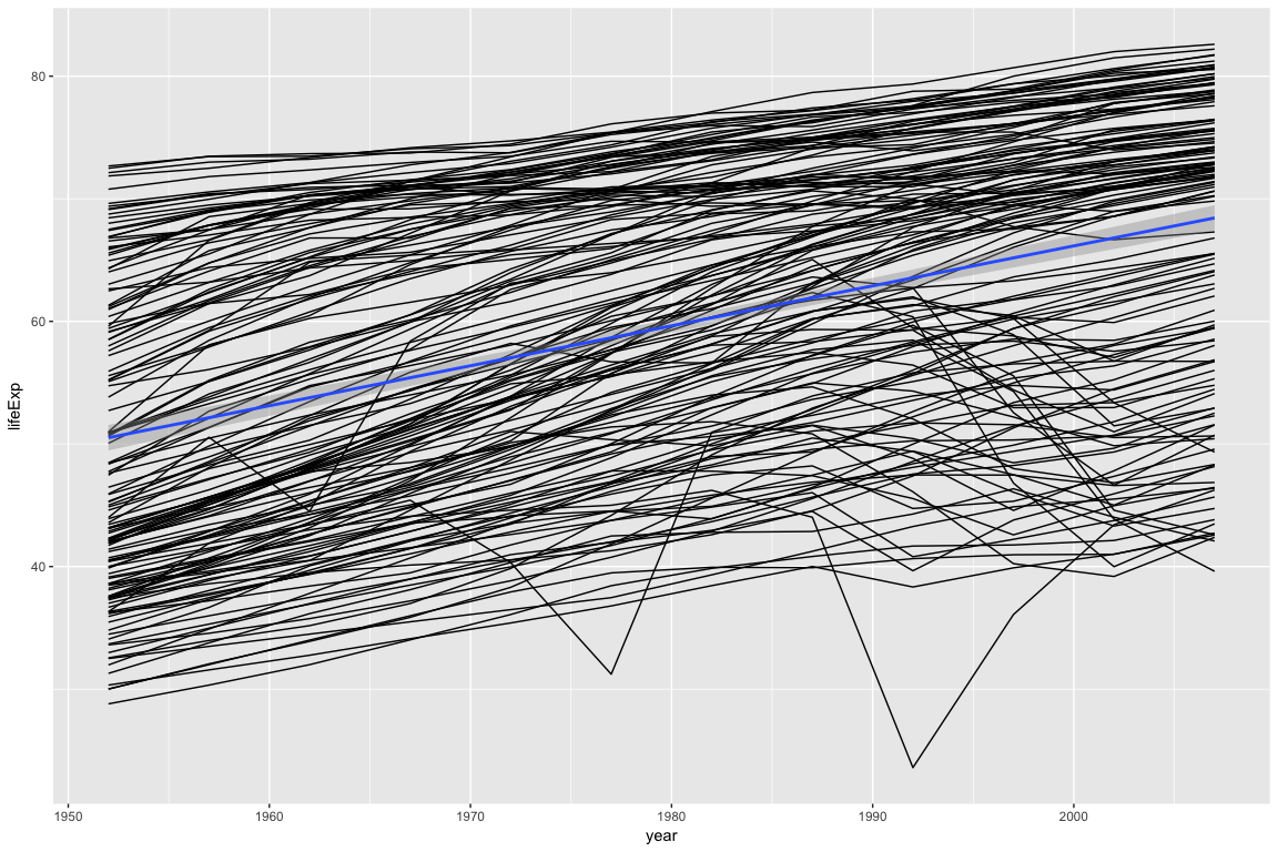
Looking at the plot above, most countries follow a linear trend: As the year increases, life expectancy goes up. A few countries do not follow a linear trend.
In the examples below, we will extract cognostics to aid in exploring the countries whose life expectancy is not linear.
trelliscopejs::facet_trelliscope()ggplot(gapminder, aes(year, lifeExp)) +
geom_smooth(method = "lm", formula = y ~ x) +
geom_line() +
trelliscopejs::facet_trelliscope(
~ country + continent,
nrow = 3, ncol = 6,
self_contained = TRUE,
auto_cog = TRUE,
state = list(
# set the state to display the country, continent, and R^2 value
# sorted by ascending R^2 value
sort = list(trelliscopejs::sort_spec("_lm_r2")),
labels = c("country", "continent", "_lm_r2")
),
path = "readme-figs/facet"
)
#> using data from the first layer
# (screen shot of trelliscopejs widget)trelliscopejs::trelliscope()This is a full, start to finish example how automatic cognostics could be inserted into a data exploration workflow.
# Find a consistent y range
y_range <- range(gapminder$lifeExp)

## # Set up data and panel column
gapminder %>%
  group_by(country, continent) %>%
  # nest the data according to the country and continent
  nest() %>%
  mutate(
    # create a column of plots with a
    # * line
    # * linear model
    panel = lapply(data, function(dt) {
      ggplot(dt, aes(year, lifeExp)) +
        geom_smooth(method = "lm", formula = y ~ x) +
        geom_line() +
        ylim(y_range[1], y_range[2])
    })
  ) %>%
  print() ->
gap_data
#> # A tibble: 142 x 4
#> # Groups:   country, continent [142]
#>    country     continent data                  panel
#>    <fct>       <fct>     <list>                <list>
#>  1 Afghanistan Asia      <tibble[,4] [12 × 4]> <gg>
#>  2 Albania     Europe    <tibble[,4] [12 × 4]> <gg>
#>  3 Algeria     Africa    <tibble[,4] [12 × 4]> <gg>
#>  4 Angola      Africa    <tibble[,4] [12 × 4]> <gg>
#>  5 Argentina   Americas  <tibble[,4] [12 × 4]> <gg>
#>  6 Australia   Oceania   <tibble[,4] [12 × 4]> <gg>
#>  7 Austria     Europe    <tibble[,4] [12 × 4]> <gg>
#>  8 Bahrain     Asia      <tibble[,4] [12 × 4]> <gg>
#>  9 Bangladesh  Asia      <tibble[,4] [12 × 4]> <gg>
#> 10 Belgium     Europe    <tibble[,4] [12 × 4]> <gg>
#> # … with 132 more rows

# Double check the plot worked...
# Look at the first panel (ggplot2 plot) of Afghanistan
gap_data$panel[[1]]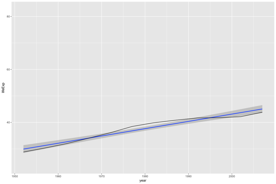
#!!!!!!!!!!
# Add cognostic information given the panel column plots
#!!!!!!!!!!
gap_data %>%
  autocogs::add_panel_cogs() %>%
  ungroup() %>%
  # double check it was added
  print(width = 100) ->
full_gap_data
#> # A tibble: 142 x 10
#>    country     continent data                  panel  `_smooth`
#>    <fct>       <fct>     <list>                <list> <list>
#>  1 Afghanistan Asia      <tibble[,4] [12 × 4]> <gg>   <tibble[,3] [1 × 3]>
#>  2 Albania     Europe    <tibble[,4] [12 × 4]> <gg>   <tibble[,3] [1 × 3]>
#>  3 Algeria     Africa    <tibble[,4] [12 × 4]> <gg>   <tibble[,3] [1 × 3]>
#>  4 Angola      Africa    <tibble[,4] [12 × 4]> <gg>   <tibble[,3] [1 × 3]>
#>  5 Argentina   Americas  <tibble[,4] [12 × 4]> <gg>   <tibble[,3] [1 × 3]>
#>  6 Australia   Oceania   <tibble[,4] [12 × 4]> <gg>   <tibble[,3] [1 × 3]>
#>  7 Austria     Europe    <tibble[,4] [12 × 4]> <gg>   <tibble[,3] [1 × 3]>
#>  8 Bahrain     Asia      <tibble[,4] [12 × 4]> <gg>   <tibble[,3] [1 × 3]>
#>  9 Bangladesh  Asia      <tibble[,4] [12 × 4]> <gg>   <tibble[,3] [1 × 3]>
#> 10 Belgium     Europe    <tibble[,4] [12 × 4]> <gg>   <tibble[,3] [1 × 3]>
#>    `_lm`            `_x`           `_y`           `_bivar`        `_n`
#>    <list>           <list>         <list>         <list>          <list>
#>  1 <tibble[,19] [1… <tibble[,5] [… <tibble[,5] [… <tibble[,2] [1… <tibble[,5] […
#>  2 <tibble[,19] [1… <tibble[,5] [… <tibble[,5] [… <tibble[,2] [1… <tibble[,5] […
#>  3 <tibble[,19] [1… <tibble[,5] [… <tibble[,5] [… <tibble[,2] [1… <tibble[,5] […
#>  4 <tibble[,19] [1… <tibble[,5] [… <tibble[,5] [… <tibble[,2] [1… <tibble[,5] […
#>  5 <tibble[,19] [1… <tibble[,5] [… <tibble[,5] [… <tibble[,2] [1… <tibble[,5] […
#>  6 <tibble[,19] [1… <tibble[,5] [… <tibble[,5] [… <tibble[,2] [1… <tibble[,5] […
#>  7 <tibble[,19] [1… <tibble[,5] [… <tibble[,5] [… <tibble[,2] [1… <tibble[,5] […
#>  8 <tibble[,19] [1… <tibble[,5] [… <tibble[,5] [… <tibble[,2] [1… <tibble[,5] […
#>  9 <tibble[,19] [1… <tibble[,5] [… <tibble[,5] [… <tibble[,2] [1… <tibble[,5] […
#> 10 <tibble[,19] [1… <tibble[,5] [… <tibble[,5] [… <tibble[,2] [1… <tibble[,5] […
#> # … with 132 more rows

# Display the panel and cognostics in a trelliscopejs widget
trelliscopejs::trelliscope(
  full_gap_data, "gapminder life expectancy",
  panel_col = "panel",
  ncol = 6, nrow = 3,
  auto_cog = FALSE,
  self_contained = TRUE,
  state = list(
    # sort by ascending R^2 value (percent explained by linear model)
    sort = list(trelliscopejs::sort_spec("_lm_r2")),
    # display the country, continent, and R^2 value
    labels = c("country", "continent", "_lm_r2")
  ),
  path = "readme-figs/manually"
)
#> New names:
#> * min -> min...26
#> * max -> max...27
#> * mean -> mean...28
#> * median -> median...29
#> * var -> var...30
#> * ...
#> Warning: Removed 4 rows containing missing values (geom_smooth).
#> Warning: Removed 8 rows containing missing values (geom_smooth).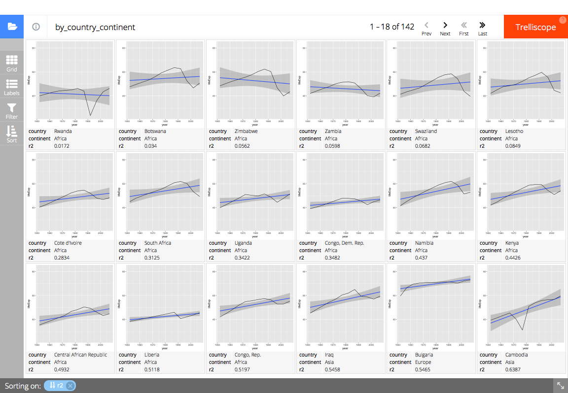
# (screen shot of trelliscopejs widget)add_cog_group() to add a custom cognostics group.add_layer_cogs() to call which cognostics groups should
be executed for a given plot layer.Using existing code from the autocogs package, we will
add the univariate continuous cognostics group.
add_cog_group(
  "univariate_continuous",
  field_info("x", "continuous"),
  "univariate metrics for continuous data",
  function(x, ...) {
    x_range <- range(x, na.rm = TRUE)
    list(
      min = cog_desc(x_range[1], "minimum of non NA data"),
      max = cog_desc(x_range[2], "maximum of non NA data"),
      mean = cog_desc(mean(x, na.rm = TRUE), "mean of non NA data"),
      median = cog_desc(median(x, na.rm = TRUE), "median of non NA data"),
      var = cog_desc(var(x, na.rm = TRUE), "variance of non NA data")
    )
  }
)
We can then call the 'univariate_continuous' cognostics
group whenever a geom_rug layer is added in a ggplot2 plot
object using the code below.
add_layer_cogs(
  # load_all(); p <- qplot(x = 1, y = Sepal.Length, data = iris, geom = "boxplot"); plot_cogs(p)
  "geom_boxplot",
  "boxplot plot",
  cog_group_df(
    "univariate_continuous", "y", "_y",
    "boxplot", "y", "_boxplot",
    "univariate_counts", "y", "_n"
  )
)