![]()
![]()
The goal of bayesROE is to provide an R package and a Shiny User Interface for easy computation and visualization of Bayesian regions of evidence as described by Hoefler and Miller (2023): Project History on Open Science Framework. Such regions of evidence (RoE) serve to systematically probe the sensitivity of a superiority or non-inferiority claim against any prior assumption of its assessors. Thus, their presentation aids research transparency and scientific evaluation of study findings.
Besides generic functions, the package also provides an intuitive user interface for a Shiny application, that can be run in a local R environment. An online version of this application is hosted on shinyapps.io: https://htaor.shinyapps.io/shinyroe
You can install the development version of bayesROE like so:
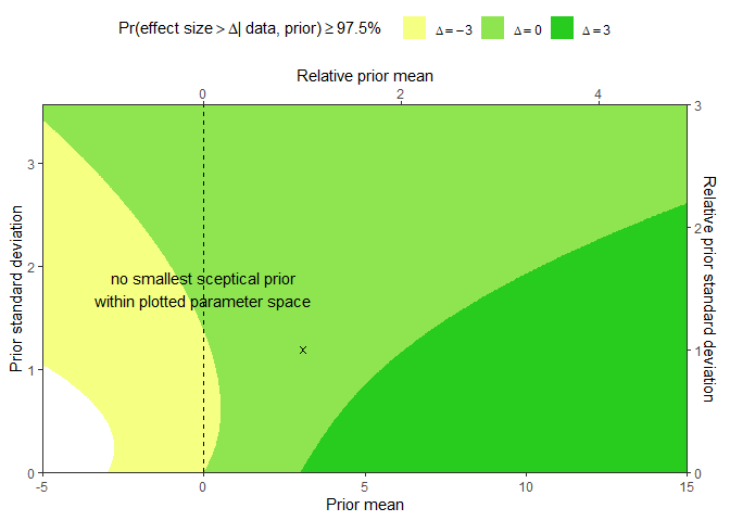
The following code extends the example from Hoefler and Miller (2023) by visualizing the RoE for one non-inferiority claim (delta = -3 pts) and the ROEs for two superiority claims (delta = 0 points and delta = 3 points) for an additional reduction of MADRS scores due to adjunct Esketamine treatment of patients suffering from moderate to severe major depression:
library(bayesROE)

# Arguments to reproduce Figure from Hoefler and Miller (2023)
init <- list(ee = 3.07, se = 1.19, delta = c(-3, 0, 3), alpha = 0.025, sceptPrior = 0)
cols <- list(col_lower = "#F5FF82", col_upper = "#27CC1E")

# Pass Arguments to Locally Run Shiny Application using run_app()
if(interactive()){
  run_app(init = init, cols = cols)
}

# Alternatively Generate and Customize Regions of Evidence Plot using ribbonROE()
HM23.3 <- ribbonROE(ee = init$ee, se = init$se, delta = init$delta, alpha = init$alpha,
                    sceptPrior = init$sceptPrior,
                    cols = c(cols$col_lower, cols$col_upper))$plot +
  ggplot2::annotate(geom = "point", y = init$ee, x = init$se, shape = 4) +
  ggplot2::coord_flip(ylim = c(-5, 15))
#> Coordinate system already present. Adding new coordinate system, which will
#> replace the existing one.
The resulting RoE plot enables to evaluate the presence of the respective claim (colored areas) or their absence (white area) as a function of prior expected mean (x-axis) and prior standard deviation (y-axis) that could be used by an assessor. The cross marks the effect estimate that was used to construct the RoE. The dashed vertical line represents all the sceptical priors that assume the true effect around 0, with a varying degree of uncertainty.