
![]()
![]()
The solution for the best-fit straight line to independent points with normally distributed errors in both x and y is known e.g. from York (1966, 1968, 2004). It provides unbiased estimates of the intercept, slope and standard errors of the best-fit straight line, even when the x and y errors are correlated.
The bfsl package implements York’s general solution and provides the best-fit straight line of bivariate data with errors in both coordinates.
Other commonly used least-squares estimation methods, such as ordinary least-squares regression, orthogonal distance regression (also called major axis regression), geometric mean regression (also called reduced major axis or standardised major axis regression) or Deming regression are all special cases of York’s solution and only valid under particular measurement conditions.
library(bfsl)
fit = bfsl(pearson_york_data)
summary(fit)
#>
#> Call:
#> bfsl.default(x = pearson_york_data)
#>
#> Residuals:
#>     Min.   1st Qu.    Median      Mean   3rd Qu.      Max.
#> -0.42396  -0.20650   0.14745   0.05573   0.34804   0.42009
#>
#> Coefficients:
#>            Estimate  Std. Error
#> Intercept   5.47991   0.29497
#> Slope      -0.48053   0.05799
#>
#> Goodness of fit: 1.483
#> Chisq-statistic: 11.87 on 8 degrees of freedom
#> Covariance of the slope and intercept: -0.01651
#> p-value: 0.1573plot(fit)
ols = bfsl(pearson_york_data, sd_x = 0, sd_y = 1)
abline(coef = ols$coef[,1], lty = 2)
legend("topright", c("best-fit straight line", "ordinary least squares"), lty = c(1,2))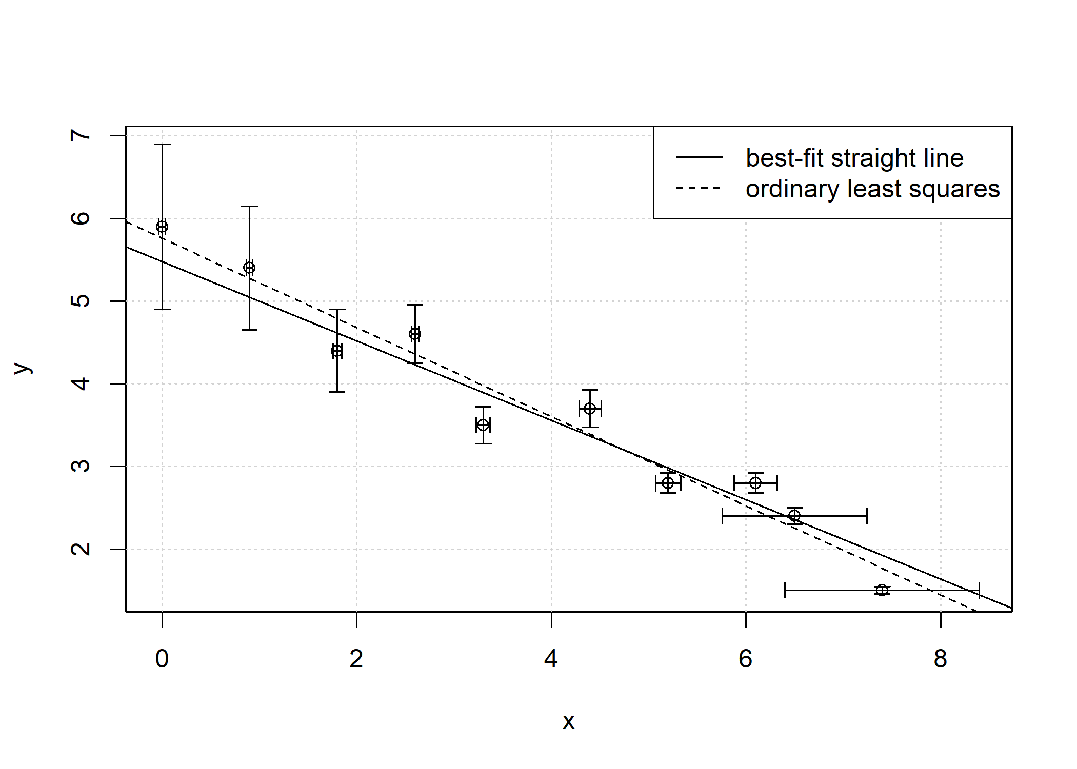
# with confidence interval
df = as.data.frame(fit$data)
newx = seq(min(df$x-df$sd_x), max(df$x+df$sd_x), length.out = 100)
preds = predict(fit, newdata = data.frame(x=newx), interval = 'confidence')

# plot
plot(y ~ x, data = df, type = 'n', xlim = c(min(x-sd_x), max(x+sd_x)),
     ylim = c(min(y-sd_y), max(y+sd_y)), las = 1)
grid()
polygon(c(rev(newx), newx), c(rev(preds[ ,3]), preds[ ,2]), col = 'grey90', border = NA)
abline(coef = fit$coef[,1], lty = 1)
points(df$x, df$y)
arrows(df$x, df$y-df$sd_y, df$x, df$y+df$sd_y, length = 0.05, angle = 90, code = 3)
arrows(df$x-df$sd_x, df$y, df$x+df$sd_x, df$y, length = 0.05, angle = 90, code = 3)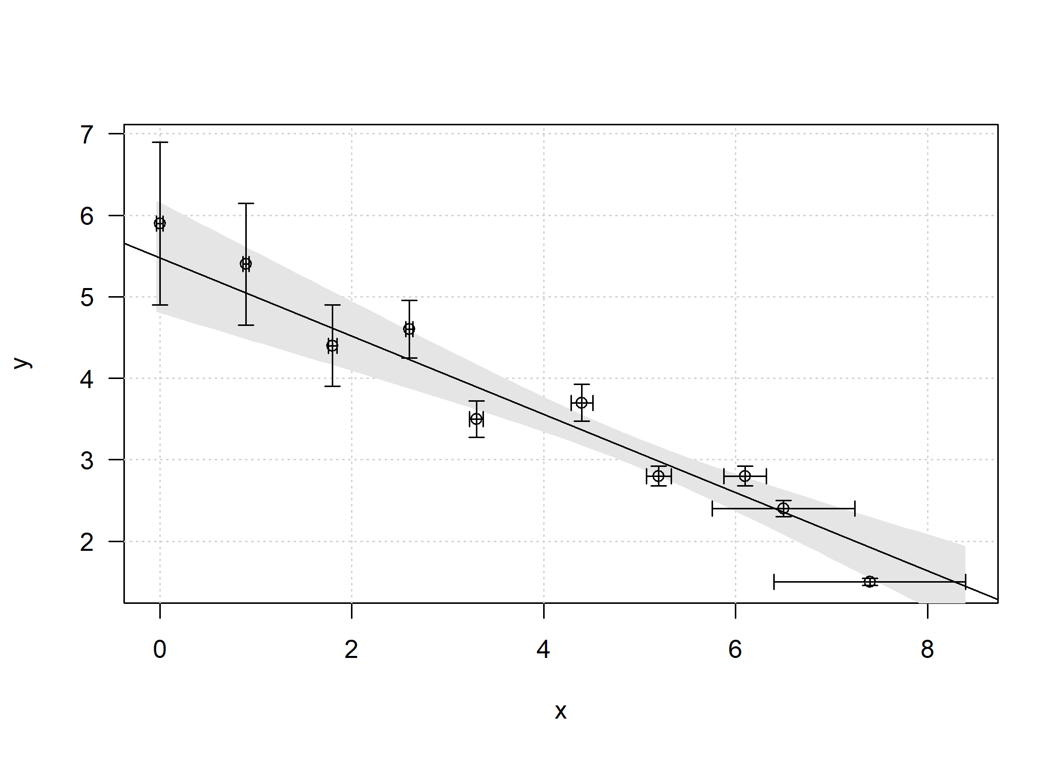
# with ggplot2
library(ggplot2)
ggplot(data = df, aes(x = x, y = y)) +
  geom_point() +
  geom_smooth(method = bfsl, method.args = list(sd_x = df$sd_x, sd_y = df$sd_y)) +
  geom_errorbar(aes(ymin = y-sd_y, ymax = y+sd_y), width = 0.05) +
  geom_errorbarh(aes(xmin = x-sd_x, xmax = x+sd_x), height = 0.05)
#> `geom_smooth()` using formula 'y ~ x'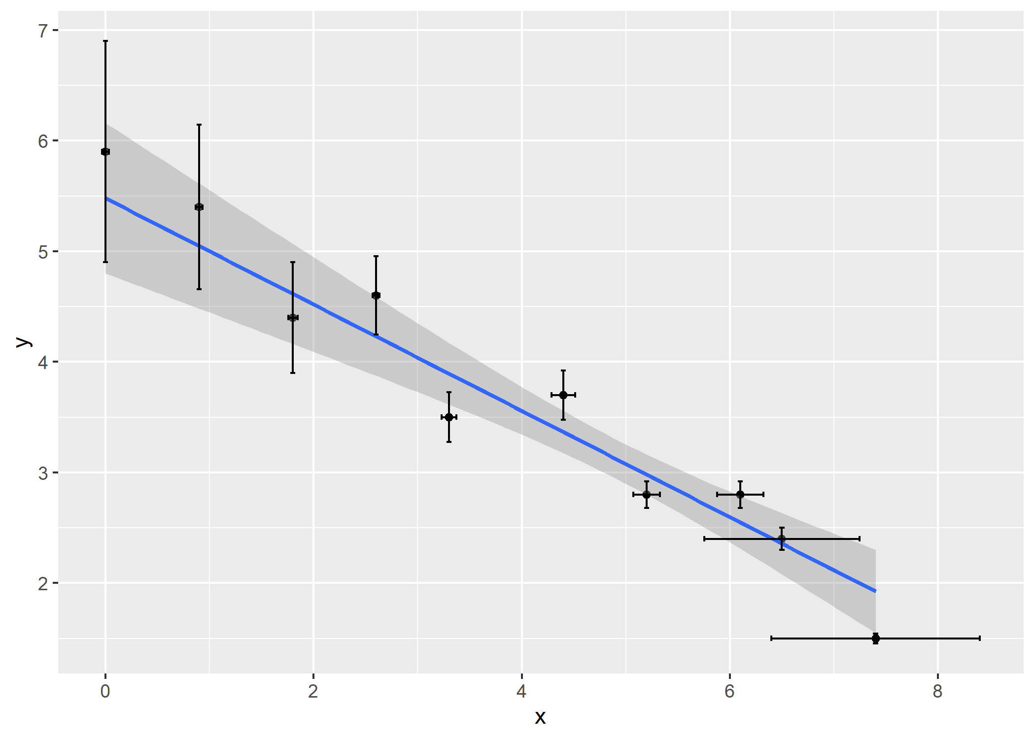
# broom tidier methods
tidy(fit, conf.int = TRUE)
#> # A tibble: 2 x 5
#>   term        estimate std.error conf.low conf.high
#>   <chr>          <dbl>     <dbl>    <dbl>     <dbl>
#> 1 (Intercept)    5.48     0.295     4.80      6.16
#> 2 Slope         -0.481    0.0580   -0.614    -0.347
glance(fit)
#> # A tibble: 1 x 7
#>   chisq p.value df.residual  nobs isConv  iter   finTol
#>   <dbl>   <dbl>       <dbl> <int> <lgl>  <dbl>    <dbl>
#> 1  1.48   0.157           8    10 TRUE       7 2.01e-11
augment(fit, newdata = data.frame(x = c(2:6)))
#> # A tibble: 5 x 3
#>       x .fitted .se.fit
#>   <int>   <dbl>   <dbl>
#> 1     2    4.52  0.185
#> 2     3    4.04  0.135
#> 3     4    3.56  0.0933
#> 4     5    3.08  0.0771
#> 5 6 2.60 0.0995Install bfsl from CRAN with:
install.packages("bfsl")Install the development version from GitHub with:
if (!require("remotes")) { install.packages("remotes") }
remotes::install_github("pasturm/bfsl")
See the NEWS file for latest release notes.
York, D. (1966). Least-squares fitting of a straight line. Canadian Journal of Physics, 44(5), 1079–1086, https://doi.org/10.1139/p66-090
York, D. (1968). Least squares fitting of a straight line with correlated errors. Earth and Planetary Science Letters, 5, 320–324, https://doi.org/10.1016/S0012-821X(68)80059-7
Williamson, J. H. (1968). Least-squares fitting of a straight line, Canadian Journal of Physics, 46(16), 1845-1847, https://doi.org/10.1139/p68-523
York, D. et al. (2004). Unified equations for the slope, intercept, and standard errors of the best straight line, American Journal of Physics, 72, 367-375, https://doi.org/10.1119/1.1632486
Cantrell, C. A. (2008). Technical Note: Review of methods for linear least-squares fitting of data and application to atmospheric chemistry problems, Atmospheric Chemistry and Physics, 8, 5477-5487, https://acp.copernicus.org/articles/8/5477/2008/
Wehr, R. and Saleska, S. R. (2017). The long-solved problem of the best-fit straight line: application to isotopic mixing lines, Biogeosciences, 14, 17-29, https://doi.org/10.5194/bg-14-17-2017