cacc:
Conjunctive Analysis of Case Configurations![]()
An R Package to compute Conjunctive Analysis of Case Configurations (CACC), Situational Clustering Tests, and Main Effects
This package contains a set of functions to conduct Conjunctive Analysis of Case Configurations (CACC) (Miethe, Hart & Regoeczi, 2008), to identify and quantify situational clustering in dominant case configurations (Hart, 2019), and to determine the main effects of specific variable values on the probabilities of outcome (Hart, Rennison & Miethe, 2017). Initially conceived as an exploratory technique for multivariate analysis of categorical data, CACC has developed to include formal statistical tests that can be applied in a wide variety of contexts. This technique allows examining composite profiles of different units of analysis in an alternative way to variable-oriented methods.
You can install the development version of cacc from GitHub with:
# Check if the`devtools` package needs to be installed
if (!require("devtools")) install.package("devtools")

# Install the {cacc} package from GitHub
devtools::install_github("amoneva/cacc")# Load {cacc} and the {tidyverse}
library(cacc)
library(tidyverse)
#> ── Attaching packages ─────────────────────────────────────── tidyverse 1.3.2 ──
#> ✔ ggplot2 3.3.6 ✔ purrr 0.3.4
#> ✔ tibble 3.1.8 ✔ dplyr 1.0.9
#> ✔ tidyr 1.2.0 ✔ stringr 1.4.1
#> ✔ readr 2.1.2 ✔ forcats 0.5.2
#> ── Conflicts ────────────────────────────────────────── tidyverse_conflicts() ──
#> ✖ dplyr::filter() masks stats::filter()
#> ✖ dplyr::lag() masks stats::lag()# Explore the dataset
onharassment |> glimpse()
#> Rows: 4,174
#> Columns: 12
#> $ sex <fct> male, male, male, female, female, female, male, female, m…
#> $ age <fct> 15-17, 18-21, 18-21, 18-21, 18-21, 15-17, 12-14, 12-14, 1…
#> $ hours <fct> 4-7, 4-7, 4-7, 4-7, 4-7, 4-7, <4, 4-7, 4-7, 4-7, <4, <4, …
#> $ snapchat <fct> yes, no, no, yes, no, yes, yes, yes, no, no, no, no, no, …
#> $ instagram <fct> yes, yes, yes, yes, yes, yes, yes, yes, yes, yes, no, yes…
#> $ facebook <fct> no, no, no, yes, no, no, no, no, no, no, no, no, no, no, …
#> $ twitter <fct> yes, yes, no, yes, no, no, no, no, no, yes, no, no, no, n…
#> $ name <fct> no, yes, no, no, yes, yes, yes, yes, yes, yes, no, yes, n…
#> $ photos <fct> no, no, no, no, no, yes, yes, yes, yes, yes, no, no, no, …
#> $ privacy <fct> no, no, no, no, no, no, no, no, no, no, no, no, no, no, n…
#> $ rep_victim <fct> 0, 0, 1, 1, 0, 1, 0, 1, 1, 0, 1, 0, 0, 0, 1, 1, 1, 0, 1, …
#> $ rep_offender <fct> 0, 0, 0, 0, 0, 1, 0, 0, 1, 0, 0, 0, 0, 0, 1, 1, 1, 0, 0, …# Calculate the CACC matrix
cacc_matrix <- onharassment |>
cacc(
ivs = sex:privacy,
dv = rep_victim
)
#> Joining, by = c("sex", "age", "hours", "snapchat", "instagram", "facebook",
#> "twitter", "name", "photos", "privacy")
# Look at the first few rows
cacc_matrix |> head()
#> # A tibble: 6 × 12
#> sex age hours snapchat insta…¹ faceb…² twitter name photos privacy freq
#> <fct> <fct> <fct> <fct> <fct> <fct> <fct> <fct> <fct> <fct> <int>
#> 1 female 15-17 4-7 yes yes no no yes yes no 11
#> 2 female 12-14 <4 no yes no no yes yes yes 10
#> 3 female 15-17 4-7 no yes no no yes yes no 16
#> 4 female 15-17 4-7 no yes no yes yes no no 10
#> 5 female 18-21 4-7 no yes no no no no yes 10
#> 6 female 18-21 4-7 no yes yes yes no no yes 10
#> # … with 1 more variable: p <dbl>, and abbreviated variable names ¹instagram,
#> # ²facebook# Compute a Chi-Square Goodness-of-Fit Test
cacc_matrix |> cluster_xsq()
#>
#> Chi-squared test for given probabilities
#>
#> data: obs
#> X-squared = 3378.2, df = 93, p-value < 2.2e-16# Compute a Situational Clustering Index (SCI)
cacc_matrix |> cluster_sci()
#> [1] 0.4505963
# Plot a Lorenz Curve to visualize the SCI
cacc_matrix |> plot_sci()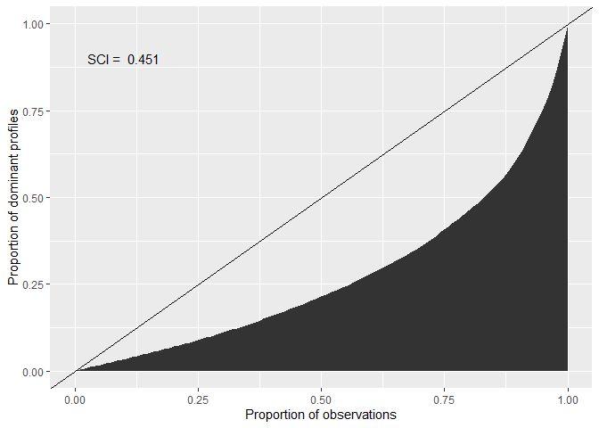
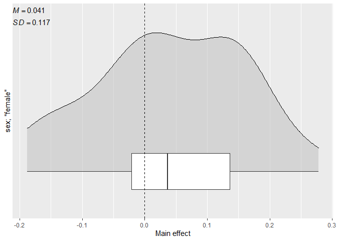
# Compute the main effects for a specific variable value
cacc_matrix |>
  main_effect(
    iv = sex,
    value = "female",
    # Set to `FALSE` for a numeric vector of effects
    summary = TRUE
  )
#> # A tibble: 1 × 5
#>   median  mean    sd    min   max
#>    <dbl> <dbl> <dbl>  <dbl> <dbl>
#> 1  0.037 0.041 0.117 -0.188 0.278

# Plot the distribution of the main effect
cacc_matrix |>
  plot_effect(
    iv = sex,
    value = "female"
  )