The purpose of dvir is to implement state-of-the-art algorithms for DNA-based disaster victim identification (DVI). In particular, dvir performs joint identification of multiple victims.
The methodology and algorithms of dvir are described in Vigeland & Egeland (2021): DNA-based Disaster Victim Identification.
The dvir package is part of the pedsuite, a collection of R packages for pedigree analysis. Much of the machinery behind dvir is imported from other pedsuite packages, especially pedtools for handling pedigree data, and forrel for the calculation of likelihood ratios. A comprehensive presentation of these packages, and much more, can be found in the book Pedigree Analysis in R.
To get the current official version of dvir, install from CRAN as follows:
install.packages("dvir")Alternatively, the latest development version may be obtained from GitHub:
# install.packages("remotes")
remotes::install_github("magnusdv/dvir")In the following we will use a toy DVI example from the paper (see above) to illustrate how to use dvir.
To get started, we load the dvir package.
library(dvir)
#> Loading required package: pedtoolsWe consider the DVI problem shown below, in which three victim samples (V1, V2, V3) are to be matched against three missing persons (M1, M2, M3) belonging to two different families.
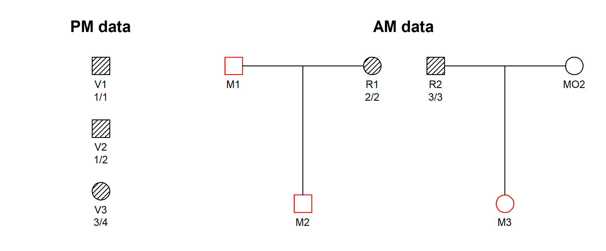
The hatched symbols indicate genotyped individuals. In this simple example we consider only a single marker, with 10 equifrequent alleles denoted 1, 2,…, 10. The available genotypes are shown in the figure.
DNA profiles from victims are generally referred to as post mortem (PM) data, while the ante mortem (AM) data contains profiles from the reference individuals R1 and R2.
A possible solution to the DVI problem is called an assignment. In our toy example, there are a priori 14 possible assignments, which can be listed as follows:
#>    V1 V2 V3
#> 1   *  *  *
#> 2   *  * M3
#> 3   * M1  *
#> 4   * M1 M3
#> 5   * M2  *
#> 6   * M2 M3
#> 7  M1  *  *
#> 8  M1  * M3
#> 9  M1 M2  *
#> 10 M1 M2 M3
#> 11 M2  *  *
#> 12 M2  * M3
#> 13 M2 M1  *
#> 14 M2 M1 M3
Each row indicates the missing persons corresponding to V1, V2 and V3
(in that order) with * meaning not identified. For
example, the first line contains the null model corresponding
to none of the victims being identified, while the last line gives the
assignment where (V1, V2, V3) = (M1, M2, M3), For each
assignment a we can calculate the likelihood, denoted
L(a). The null likelihood is denoted L0.
We consider the following to be two of the main goals in the analysis of a DVI case with multiple missing persons:
a to
the null model: LR = L(a)/L0.P(Vi = Mj | data) for all combinations of i and j, and the
posterior non-pairing probabilities
P(Vi = '*' | data) for all i.The pedigrees and genotypes for this toy example are available within
dvir as a built-in dataset, under the name
example2.
example2
#> DVI dataset:
#>  3 victims (2M/1F): V1, V2, V3
#>  3 missing (2M/1F): M1, M2, M3
#>  2 typed refs: R1, R2
#>  2 ref families: 1, 2
#> Number of markers, PM and AM: 1
Internally, all DVI datasets in dvir have the
structure of a list, with elements pm (the victim data),
am (the reference data) and missing (a vector
naming the missing persons): We can inspect the data by printing each
object. For instance, in this case am is a list of two
pedigrees:
example2$am
#> [[1]]
#>  id fid mid sex  L1
#>  M1   *   *   1 -/-
#>  R1   *   *   2 2/2
#>  M2  M1  R1   1 -/-
#>
#> [[2]]
#>   id fid mid sex  L1
#>   R2   *   *   1 3/3
#>  MO2   *   *   2 -/-
#>   M3  R2 MO2   2 -/-
Note that the two pedigrees are printed in so-called ped
format, with columns id (ID label), fid
(father), mid (mother), sex (1 = male; 2 =
female) and L1 (genotypes at locus L1).
The code generating this dataset can be found in the github repository of dvir, more specifically here: https://github.com/magnusdv/dvir/blob/master/data-raw/example2.R.
A great way to inspect a DVI dataset is to plot it with the function
plotDVI().
plotDVI(example2)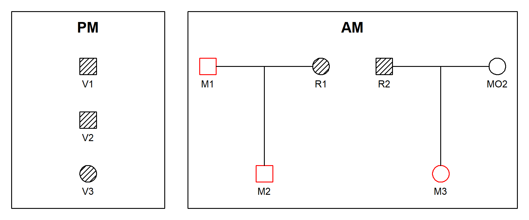
The plotDVI() function offers many parameters for
tweaking the plot; see the help page ?plotDVI() for
details.
The jointDVI() function performs joint identification of
all three victims, given the data. It returns a data frame ranking all
assignments with nonzero likelihood:
jointRes = jointDVI(example2, verbose = FALSE)

# Print the result
jointRes
#>    V1 V2 V3    loglik  LR   posterior
#> 1  M1 M2 M3 -16.11810 250 0.718390805
#> 2  M1 M2  * -17.72753  50 0.143678161
#> 3   * M2 M3 -18.42068  25 0.071839080
#> 4  M1  * M3 -20.03012   5 0.014367816
#> 5   * M1 M3 -20.03012   5 0.014367816
#> 6   * M2  * -20.03012   5 0.014367816
#> 7   *  * M3 -20.03012   5 0.014367816
#> 8  M1  *  * -21.63956   1 0.002873563
#> 9   * M1  * -21.63956   1 0.002873563
#> 10  *  *  * -21.63956   1 0.002873563
The output shows that the most likely joint solution is (V1, V2, V3) = (M1, M2, M3), with an LR of 250 compared to the null model.
The function plotSolution() shows the most likely
solution:
plotSolution(example2, jointRes, marker = 1)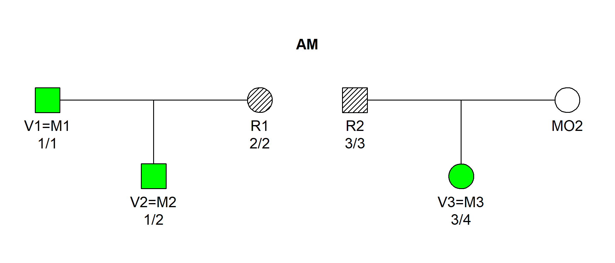
By default, the plot displays the assignment in the first row of
jointRes. To examine the second most likely, add
k = 2 (and so on to go further down the list).
Next, we compute the posterior pairing (and non-pairing)
probabilities. This is done by feeding the output from
jointDVI() into the function Bmarginal().
Bmarginal(jointRes, example2$missing, prior = NULL)
#>            M1        M2        M3          *
#> V1 0.87931034 0.0000000 0.0000000 0.12068966
#> V2 0.01724138 0.9482759 0.0000000 0.03448276
#> V3 0.00000000 0.0000000 0.8333333 0.16666667
Here we used a default flat prior for simplicity, assigning equal prior probabilities to all assignments.
we see that the posterior pairing probabilities for the most likely solution are