![]()
emstreeR enables R users to fast and easily compute an Euclidean Minimum Spanning Tree (EMST) from data. This package relies on the R API for {mlpack} - the C++ Machine Learning Library (Curtin et. al., 2013). {emstreeR} uses the Dual-Tree Boruvka (March, Ram, Gray, 2010, https://doi.org/10.1145/1835804.1835882), which is theoretically and empirically the fastest algorithm for computing an EMST. This package also provides functions and an S3 method for readily plotting Minimum Spanning Trees (MST) using either the style of the {base}, {scatterplot3d}, or {ggplot2} libraries; and functions to export the MST output to shapefiles.
computeMST() computes an Euclidean Minimum Spanning Tree for the input data.plot.MST() an S3 method for the generic function plot() that produces 2D MST plots.plotMST3D() plots a 3D MST using the {scatterplot3d} style.stat_MST() a {ggplot2} Stat extension for plotting a 2D MST.export_vertices_to_shapefile() writes a shapefile containing the MST vertices.export_edges_to_shapefile() writes a shapefile containing the MST edges.# CRAN version
install.packages("emstreeR")
# Dev version
if (!require('devtools')) install.packages('devtools')
devtools::install_github("allanvc/emstreeR")## artificial data:
set.seed(1984)
n <- 7
c1 <- data.frame(x = rnorm(n, -0.2, sd = 0.2), y = rnorm(n, -2, sd = 0.2))
c2 <- data.frame(x = rnorm(n, -1.1, sd = 0.15), y = rnorm(n, -2, sd = 0.3))
d <- rbind(c1, c2)
d <- as.data.frame(d)
## MST:
library(emstreeR)
out <- ComputeMST(d)
out## x y from to distance
## 1 -0.118159357 -2.166545 11 13 0.03281747
## 2 -0.264604994 -2.105242 8 12 0.05703382
## 3 -0.072829535 -1.716803 3 7 0.08060398
## 4 -0.569225757 -1.943598 5 6 0.11944501
## 5 -0.009270527 -1.942413 6 7 0.13450475
## 6 0.037697969 -1.832590 8 10 0.14293342
## 7 -0.091509110 -1.795213 1 2 0.15875908
## 8 -1.097338236 -1.871078 10 14 0.16993335
## 9 -0.841400898 -2.194585 1 5 0.24918237
## 10 -1.081888729 -1.728982 8 13 0.27882008
## 11 -1.366334073 -2.003965 2 4 0.34485145
## 12 -1.081078171 -1.925745 9 12 0.36016689
## 13 -1.357063682 -1.972485 4 9 0.37023475
## 14 -0.913706515 -1.753315 1 1 0.00000000## artifical data for 2D plots:
set.seed(1984)
n <- 15
c1 <- data.frame(x = rnorm(n, -0.2, sd = 0.2), y = rnorm(n, -2, sd = 0.2))
c2 <- data.frame(x = rnorm(n, -1.1, sd = 0.15), y = rnorm(n, -2, sd = 0.3))
d <- rbind(c1, c2)
d <- as.data.frame(d)
## MST:
library(emstreeR)
out <- ComputeMST(d, verbose = FALSE)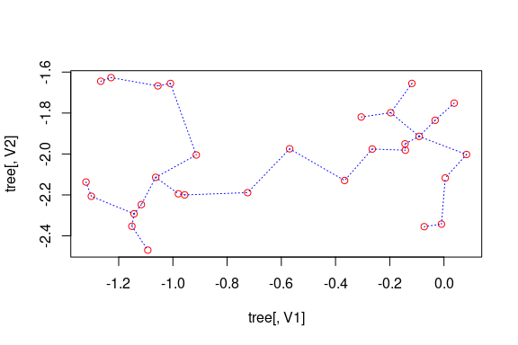
## 2D plot with ggplot2:
library(ggplot2)
ggplot(data = out, aes(x = x, y = y, from = from, to = to))+
  geom_point()+
  stat_MST(colour="red")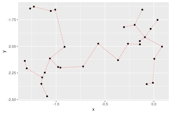
## 2D curved edges plot with ggplot2:
library(ggplot2)
ggplot(data = out, aes(x = x, y = y, from = from, to = to))+
  geom_point()+
  stat_MST(geom="curve")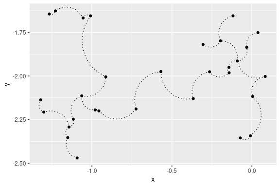
## artificial data for 3D plots:
n = 99
set.seed(1984)
d1 <- matrix(rnorm(n, mean = -2, sd = .5), n/3, 3) # 3d
d2 <- matrix(rnorm(n, mean = 0, sd = .3), n/3, 3)
d3 <- matrix(rnorm(n, mean = 3, sd = .4), n/3, 3)
d <- rbind(d1,d2,d3) # showing a matrix input

## MST:
library(emstreeR)
out <- ComputeMST(d, verbose = FALSE)
## simple 3D plot:
plotMST3D(out, xlab = "xaxis", col.pts = "orange", col.segts = "red", main = "a simple MST 3D plot")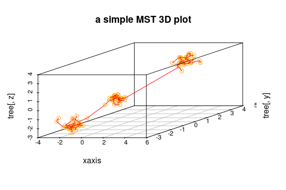
## mock data
country_coords_txt <- "
1 3.00000 28.00000 Algeria
2 54.00000 24.00000 UAE
3 139.75309 35.68536 Japan
4 45.00000 25.00000 'Saudi Arabia'
5 9.00000 34.00000 Tunisia
6 5.75000 52.50000 Netherlands
7 103.80000 1.36667 Singapore
8 124.10000 -8.36667 Korea
9 -2.69531 54.75844 UK
10 34.91155 39.05901 Turkey
11 -113.64258 60.10867 Canada
12 77.00000 20.00000 India
13 25.00000 46.00000 Romania
14 135.00000 -25.00000 Australia
15 10.00000 62.00000 Norway"
d <- read.delim(text = country_coords_txt, header = FALSE,
quote = "'", sep = "",
col.names = c('id', 'lon', 'lat', 'name'))
## MST
library(emstreeR)
output <- ComputeMST(d[,2:3])
#plot(output)
export_vertices_to_shapefile(output, file="vertices.shp")
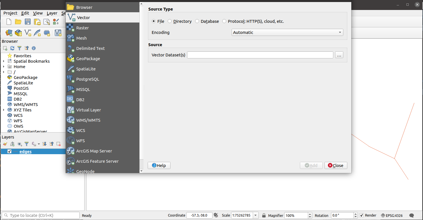
export_edges_to_shapefile(output, file="edges.shp")Below is an example of how to open the shapefiles using the QGIS software in Ubuntu.
Open file vertices.shp or edges.shp.


Then go to Menu > Layer > Add Layer > Add Vector Layer.

Select Source Type as File if it is not selected yet. Then click on the three dots button under Source to select the other shapefile, depending on which one you used to open QGIS. In the example below, we select vertices.shp as we chose edges.shp first.
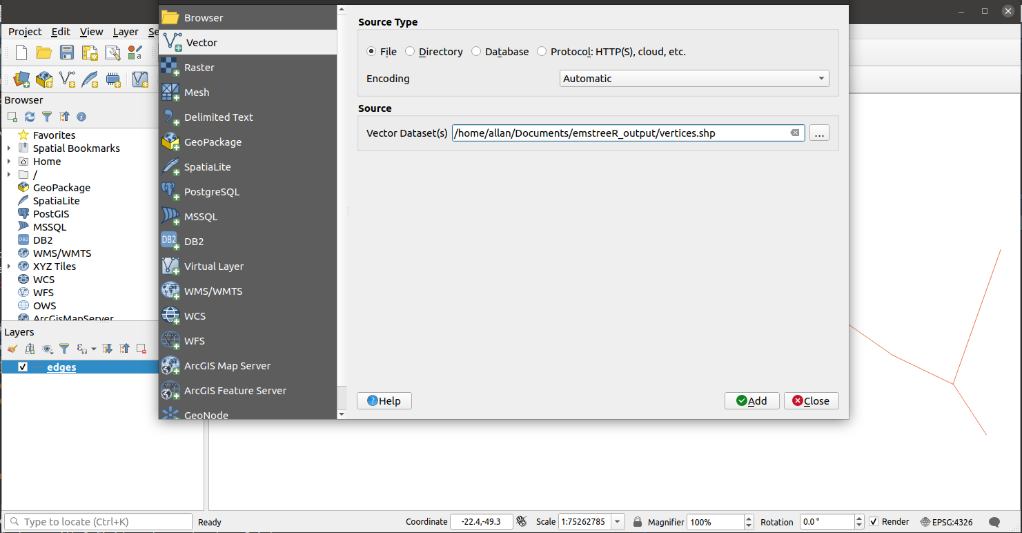
Hit Add, then Close and voilà.
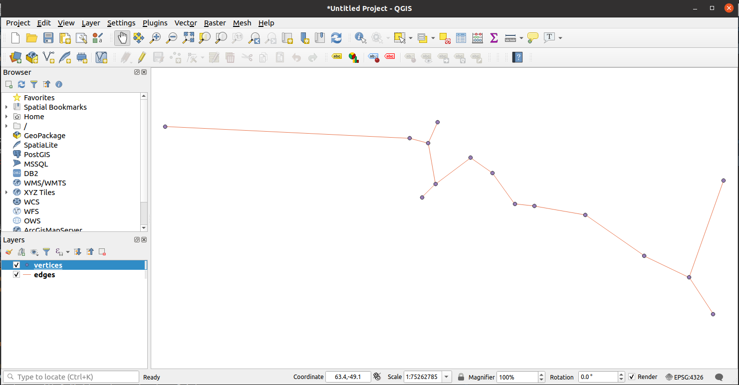
It is then very straightforward to add other layers such map shapefiles or add the generated EMST to existing layers.
This package is licensed under the terms of the BSD 3-clause License.
March, W. B., and Ram, P., and Gray, A. G. (2010). Fast euclidian minimum spanning tree: algorithm analysis, and applications. 16th ACM SIGKDD International Conference on Knowledge Discovery and Data mining, July 25-28 2010. Washington, DC, USA.
Curtin, R. R. et al. (2013). Mlpack: A scalable C++ machine learning library. Journal of Machine Learning Research, v. 14, 2013.