A lightweight R package for computing the Maximal Overlap Discrete Wavelet Transform (MODWT) and À Trous DWT. This package was originally developed to aid forecasting research in water resources (streamflow forecasting, urban water demand forecasting, etc.)
You can install the latest version of fastWavelets with
install.packages("fastWavelets")You can also install the development version of fastWavelets from GitHub with:
# install.packages("devtools")
devtools::install_github("johnswyou/fastWavelets")Here we decompose a white noise series using MODWT:
library(fastWavelets)

set.seed(839)                       # make this example reproducible

N <- 1000                           # number of time series points
J <- 4                              # decomposition level
wavelet <- 'coif1'                  # scaling filter
X <- matrix(rnorm(N),N,1)           # white noise
modwt.X <- mo_dwt(X,wavelet,J)
colnames(modwt.X) <- c(paste0("W", 1:J), paste0("V", J))
nbc <- n_boundary_coefs(wavelet, J) # number of boundary affected coefficients

# Visualizations
plot.ts(X, main = "White noise series", ylab="")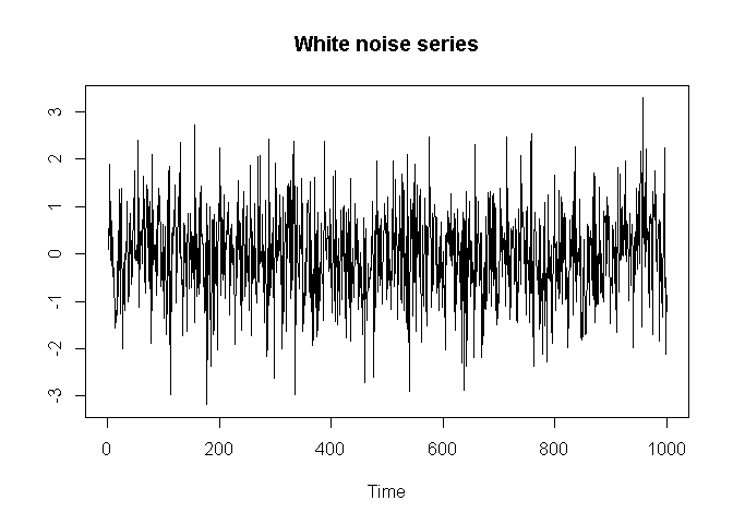
plot.ts(modwt.X, nc=1, main="MODWT coefficients")
abline(v=nbc, lwd=2, col="blue", lty=2)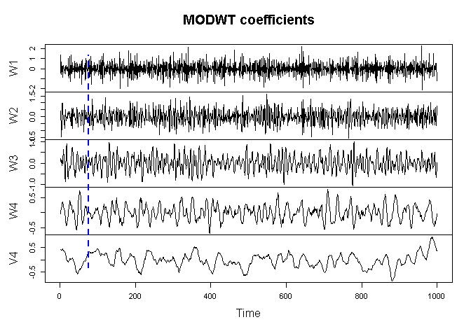
In the context of forecasting, everything to the left of the vertical dashed blue line would be removed prior to training a forecasting model using the MODWT coefficients. It is often useful to view wavelet decomposition methods such as the MODWT as a “feature generation” or “feature engineering” method.
For atrous_dwt, the set of possible values for the
argument wavelet is as follows:
c("haar", "d1", "sym1", "bior1.1", "rbio1.1",
"d2", "sym2", "d3", "sym3", "d4", "d5", "d6", "d7", "d8", "d9", "d10", "d11",
"sym4", "sym5", "sym6", "sym7", "sym8", "sym9", "sym10",
"coif1", "coif2", "coif3", "coif4", "coif5",
"bior1.3", "bior1.5", "bior2.2", "bior2.4", "bior2.6", "bior2.8", "bior3.1", "bior3.3",
"bior3.5", "bior3.7", "bior3.9", "bior4.4", "bior5.5", "bior6.8",
"rbio1.3", "rbio1.5", "rbio2.2", "rbio2.4", "rbio2.6", "rbio2.8", "rbio3.1", "rbio3.3",
"rbio3.5", "rbio3.7", "rbio3.9", "rbio4.4", "rbio5.5", "rbio6.8",
"la8", "la10", "la12", "la14", "la16", "la18", "la20",
"bl14", "bl18", "bl20",
"fk4", "fk6", "fk8", "fk14", "fk18", "fk22",
"b3spline",
"mb4.2", "mb8.2", "mb8.3", "mb8.4", "mb10.3", "mb12.3", "mb14.3", "mb16.3", "mb18.3", "mb24.3", "mb32.3",
"beyl",
"vaid",
"han2.3", "han3.3", "han4.5", "han5.5")
and for mo_dwt, the set of possible values for
wavelet is
c("haar", "d1", "sym1",
"d2", "sym2", "d3", "sym3", "d4", "d5", "d6", "d7", "d8", "d9", "d10", "d11",
"sym4", "sym5", "sym6", "sym7", "sym8", "sym9", "sym10",
"coif1", "coif2", "coif3", "coif4", "coif5",
"la8", "la10", "la12", "la14", "la16", "la18", "la20",
"bl14", "bl18", "bl20",
"fk4", "fk6", "fk8", "fk14", "fk18", "fk22",
"mb4.2", "mb8.2", "mb8.3", "mb8.4", "mb10.3", "mb12.3", "mb14.3", "mb16.3", "mb18.3", "mb24.3", "mb32.3",
"beyl",
"vaid",
"han2.3", "han3.3", "han4.5", "han5.5")Quilty, J., & Adamowski, J. (2018). Addressing the incorrect usage of wavelet-based hydrological and water resources forecasting models for real-world applications with best practices and a new forecasting framework. Journal of Hydrology, 563, 336–353. https://doi.org/10.1016/j.jhydrol.2018.05.003
Bašta, M. (2014). Additive decomposition and boundary conditions in wavelet-based forecasting approaches. Acta Oeconomica Pragensia, 22(2), 48–70. https://doi.org/10.18267/j.aop.431
Benaouda, D., Murtagh, F., Starck, J.-L., & Renaud, O. (2006). Wavelet-based nonlinear multiscale decomposition model for electricity load forecasting. Neurocomputing, 70(1-3), 139–154. https://doi.org/10.1016/j.neucom.2006.04.005
Maheswaran, R., & Khosa, R. (2012). Comparative study of different wavelets for hydrologic forecasting. Computers & Geosciences, 46, 284–295. https://doi.org/10.1016/j.cageo.2011.12.015