fitHeavyTail

Robust estimation methods for the mean vector, scatter matrix, and covariance matrix (if it exists) from data (possibly containing NAs) under multivariate heavy-tailed distributions such as angular Gaussian (via Tyler’s method), Cauchy, and Student’s t distributions. Additionally, a factor model structure can be specified for the covariance matrix. The latest revision also includes the multivariate skewed t distribution.

Installation

The package can be installed from CRAN or GitHub:

# install stable version from CRAN
install.packages("fitHeavyTail")

# install development version from GitHub
devtools::install_github("convexfi/fitHeavyTail")

To get help:

library(fitHeavyTail)
help(package = "fitHeavyTail")
?fit_mvt

To cite fitHeavyTail in publications:

citation("fitHeavyTail")

Quick Start

To illustrate the simple usage of the package fitHeavyTail, let’s start by generating some multivariate data under a Student’s \(t\) distribution with significant heavy tails (degrees of freedom \(\nu=4\)):

library(mvtnorm)  # package for multivariate t distribution
N <- 10   # number of variables
T <- 80   # number of observations
nu <- 4   # degrees of freedom for heavy tails

set.seed(42)
mu <- rep(0, N)
U <- t(rmvnorm(n = round(0.3*N), sigma = 0.1*diag(N)))
Sigma_cov <- U %*% t(U) + diag(N)  # covariance matrix with factor model structure
Sigma_scatter <- (nu-2)/nu * Sigma_cov
X <- rmvt(n = T, delta = mu, sigma = Sigma_scatter, df = nu)  # generate data

We can first estimate the mean vector and covariance matrix via the traditional sample estimates (i.e., sample mean and sample covariance matrix):

mu_sm     <- colMeans(X)
Sigma_scm <- cov(X)

Then we can compute the robust estimates via the package fitHeavyTail:

library(fitHeavyTail)
fitted <- fit_mvt(X)

We can now compute the estimation errors and see the significant improvement:

sum((mu_sm     - mu)^2)
#> [1] 0.2857323
sum((fitted$mu - mu)^2)
#> [1] 0.1487845

sum((Sigma_scm  - Sigma_cov)^2)
#> [1] 5.861138
sum((fitted$cov - Sigma_cov)^2)
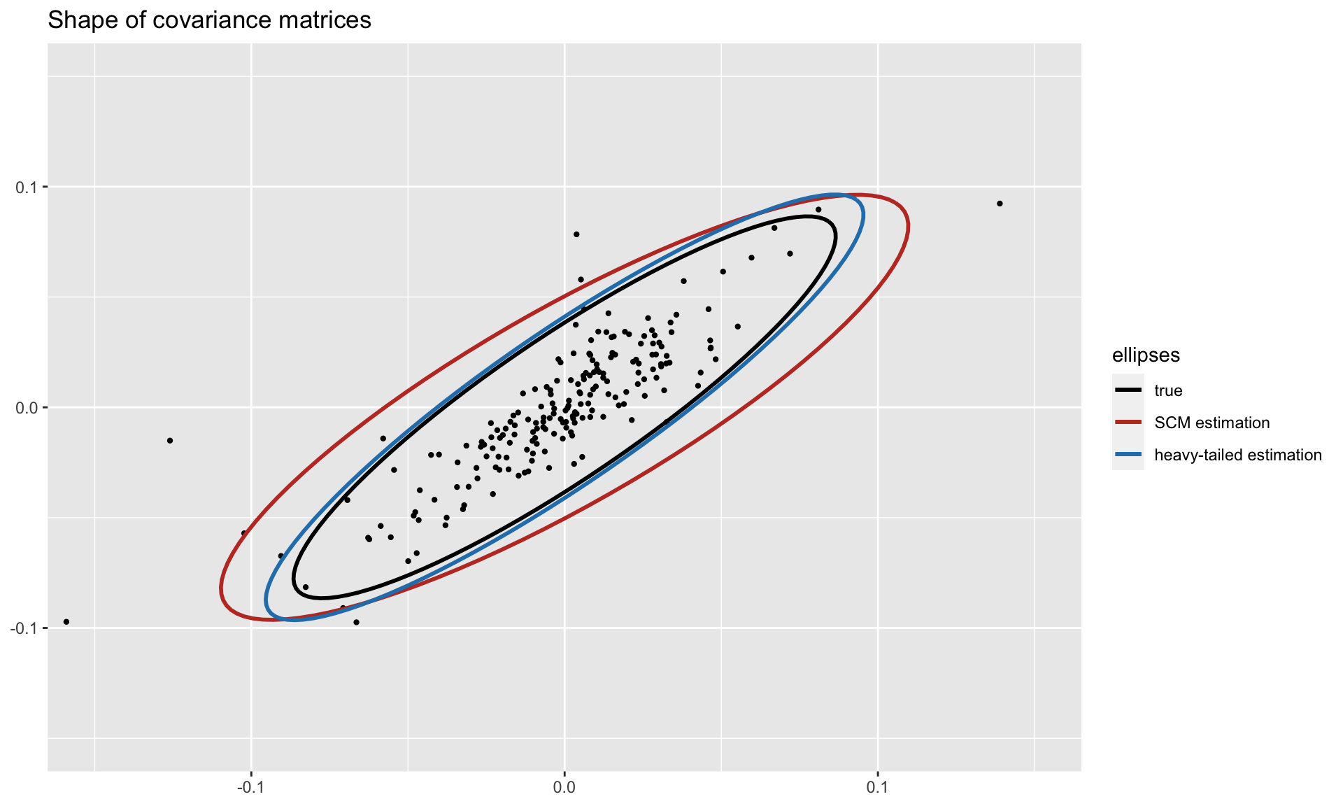
#> [1] 4.663539

To get a visual idea of the robustness, we can plot the shapes of the covariance matrices (true and estimated ones) on two dimensions. Observe how the heavy-tailed estimation follows the true one more closely than the sample covariance matrix:

Documentation

For more detailed information, please check the vignette.

Links

Package: CRAN and GitHub.

README file: GitHub-readme.

Vignette: CRAN-vignette and GitHub-vignette.