geomerge provides a framework for integration of
different types of spatial data in R. In practice, research involving
spatial data typically entails drawing on multiple sources that provide
information on distinct variables, each with a particular geographical
resolution. Conducting analysis requires integrating these variables
from the separate datasets into a common data frame, with a geographical
resolution that is appropriately comparable across all the
variables.
The main challenge is that datasets can have very different spatial
data formats. For example, information on population or elevation is
most often available as Raster data. Information on a
country’s administrative subdivisions is typically provided as
Polygon data. The locations of conflict events or incidents
of crime are usually coded as Point data. In essence, these
data formats correspond to different units of observation. Different
units implies a spatial mismatch. When spatial data are mismatched, they
may not be usable for particular types of analysis (unless purposely
considering variables at different units of observation). Separate
datasets may also treat the same variable as being of different types
(e.g., numeric vs. categorical).
There exist a whole range of packages in R providing
excellent functionality for dealing with these data integration problems
but without a single, simple framework that combines all this
functionality. In addition, integrating different kinds of spatial data
requires making assumptions and providing specifications for how to
proceed with the integration. The geomerge package provides
this framework and makes it easy to correctly make these choices and
make them explicit. The package allows for the automatic, flexible,
transparent, reproducible integration of the most common types of
spatial data. The integration can produce variables with the same
spatial resolution, or merely establish the spatial correspondence of
variables with different resolutions. In doing so, the package
implements a number of established best practices that ensure robust
results for many standard cases, while allowing for customization
through optional parameters.
Specifically, geomerge supports empirical research using
spatial data in several important ways. First, the package streamlines
the process of integrating data from multiple sources. Second, the
package offers the flexibility of enabling users to generate variants of
the same data. Each of these variants can reflect different assumptions
about how to perform the integration, including in reference to the
choice of spatial unit, as well as the choice of assignment, zonal
function or point aggregation rules. Third, the variants can be used to
test the robustness of analyses to assumptions about data integration.
Fourth, the package contributes to transparency and simplifies
replication by providing clear, standardized interfaces that document
the assumptions users made when integrating data. The data and code used
in performing any integration can be supplied to accompany similar code
used in performing analysis.
The package can be installed through the CRAN repository.
install.packages("geomerge")Or the development version from Github
# install.packages("devtools")
devtools::install_github("kdonnay/geomerge")In the following illustrations, we use a number of different data
layers for Nigeria 2011 that constitute the example data distributed
with the geomerge package. The data can be easily loaded
using
data(geomerge)The example datasets cover all three main spatial data types discussed above:
ACLED (Point data): Conflict events for
Nigeria in 2011 as recorded by the Armed Conflict Location & Event
Data project, available from https://acleddata.com/. This dataset contains geocoded,
timestamped information on individual conflict events.
AidData (Point data, including
locations geocoded to administrative divisions, but assigned coordinates
of centroids): Activities of development aid projects in Nigeria with
start dates in 2011 as recorded by AidData, available at https://www.aiddata.org/. This dataset contains
geocoded, timestamped information on individual aid projects.
Note: Both Point datasets are time-stamped, which means
that they can be used for dynamic (i.e., spanning a spatial panel) as
well as static (i.e., cross-sectional) integration.
geoEPR (Polygons data): All politically
relevant ethnic groups for Nigeria in 2011, as recorded in the EPR-Core
2014 dataset, available at https://icr.ethz.ch/data/epr/geoepr/. This dataset
assigns every politically relevant ethnic group one of six settlement
patterns and provides polygons describing their location.
gpw (Raster data): Population at a
gridded resolution of about 4km for Nigeria in 2010, as compiled by
CIESIN, available at https://sedac.ciesin.columbia.edu/data/collection/gpw-v4.
This dataset provides population estimates at several grid
resolutions.
states (Polygons data): Second-order
administrative divisions (ADM2s) for Nigeria, known as Local Government
Areas (equivalent of US states). The dataset is available at http://www.arcgis.com/home/item.html?id=0e58995046b74254911c1dc0eb756fa4.
This dataset is used in the illustration for the target
SpatialPolygonsDataFrame to which spatial data are merged. The polygons
in states have been simplified to reduce the size of the
SpatialPolygonsDataFrame and enable fast execution of the
examples provided.
The main functionality of the geomerge package is
provided by a single function with the same name. The output of the
function is an object of class “geomerge”, which is a list with three
slots: (1) data contains the spatial data resulting from
integration, (2) inputData stores the input dataset, and
(3) parameters logs all parameters with which
geomerge was executed.
Running geomerge has two basic requirements.
The first requirement is input data, comprised of any number of
objects of type SpatialPolygonsDataFrame,
SpatialPointsDataFrame and RasterLayer. The
RasterLayer will always by definition be single-valued.
Therefore, geomerge requires the user to select one
specific variable in each of the SpatialPolygonsDataFrame
and SpatialPointsDataFrame objects prior to integration.
Note that the package accepts the short-hand variable specification
using the standard “$” notation to denote the selection of a specific
variable. If dynamic integration of a
SpatialPointsDataFrame is run, a second column named
timestamp is required in the data.
The package then uses the name of the input data to label the corresponding variables in the integrated data. This approach establishes a clear, unique link between the input and integrated data. If a user wishes to work with several variables from the same dataset, simply enter these as separate arguments. We generally advise users to rely on meaningful names when labeling input data.
The second requirement, called target, specifies the
spatial structure to which variables from all input objects are merged.
The example in the geomerge package requires this
target to be of class
SpatialPolygonsDataFrame. In practice, the spatial
structure can have any shape (e.g., polygons of administrative units,
raster cells, etc.).
Note: The package provides a useful helper function called
generateGrid, which generates a grid of user-specified cell
size for the spatial extent defined by a spatial R
object.
geomerge assumes that all inputs of type
SpatialPolygonsDataFrame and RasterLayer are
static and contemporary. If the polygons or raster are changing, we
advise users to rerun geomerge for each interval in which
data are static and contemporary. The package allows for dynamic
integration of all inputs that are a
SpatialPointsDataFrame. For example, one can automatically
generate the counts of events that occur within a specific unit of
target within a specific time period.
geomerge has a number of other optional arguments, which
we will explore further below. These optional arguments enable specific
kinds of integration (i.e., dynamic vs. static) and/or allow the user to
change assumptions about zonal functions, assignment rules, etc. from
the default values.
Note: The print, summary and
plot functions are overloaded for objects of class
“geomerge”, meaning that these functions return specific outputs for
objects of class “geomerge”.
The simplest case is that of merging static layers. Consider, for
example, the case that geo-spatial information about the settlement
areas of ethnic groups ought to be merged with the administrative units
of a country to determine which group is the dominant faction in each
area. In the following examples, we therefore assume that the
target of integration is the states
SpatialPolygonsDataFrame.
We begin by integrating one Polygon dataset with
states. Note that the function returns a number of messages
documenting the progress of the integration task. When merging more
complex data, the function may run for some time and monitoring progress
can therefore be relevant. If no printed progress updates are required,
simply use the optional argument silent = TRUE; for all our
illustrations we will use this to suppress the R console
output.
output = geomerge(geoEPR,target=states,silent=TRUE)## Loading required namespace: rgeossummary (output)## geomerge completed: 1 datasets successfully integrated - run in static mode.
##
## The following 1 non numerical variable(s) are available:
## geoEPR
##
## First and second order spatial lag values available.names(output$data)## [1] "FID" "ID" "NAME_0" "NAME_1" "area" "geoEPR"Here, the default settings of geomerge make implicit
assumptions regarding the assignment of the values in
geoEPR to the target of states
SpatialPolygonsDataFrame. The default assignment rule uses
maximum area overlap (assignment = "max(area)"). This rule
implies that a value is assigned to any spatial unit of
target that corresponds to the unit in geoEPR
with the largest spatial overlap.
As an alternative, geomerge supports assignment based on
minimal area overlap (assignment = "min(area)").
Assignment can also be done by maximum population
(assignment ="max(pop)") or minimum population
assignment = "min(pop)"), which operate similar to the area
.
In addition, geomerge permits assignment weighted by
area (assignment= "weighted(area)") or population
(assignment = "weighted(pop)"). The former assigns the
value that is the area-weighted average across all units intersecting
with the spatial unit in target. The latter is analogous,
but assigns the value based on the population represented by that
area.
Naturally, all the options relying on population require a population
raster input called population.data. Here is an
example:
output = geomerge(geoEPR,target=states,assignment="max(pop)",
                  population.data=gpw, silent=TRUE)
summary (output)
## geomerge completed: 1 datasets successfully integrated - run in static mode.
##
## The following 1 non numerical variable(s) are available:
## geoEPR
##
## First and second order spatial lag values available.Note: Any weighted assignment (whether area- or population-based) is
only allowed for numeric data. Within our illustration, therefore,
weighted assignment is not possible for the layer
geoEPR.
The integration of Raster data is similarly
straightforward.
Note: geomerge accepts any optional arguments of the
function extract in the raster package. These
arguments can be entered in the exact same syntax as in the original
extract function and are passed on to any use of the
function within the package. For example, in the illustration we use the
optional input na.rm = TRUE because the gpw
data has a few missing values that we want to ignore when performing the
data integration.
output = geomerge(gpw,na.rm=TRUE,target=states,silent=TRUE)
summary (output)
## geomerge completed: 1 datasets successfully integrated - run in static mode.
##
## The following 1 numerical variable(s) are available:
## gpw
##
## First and second order spatial lag values available.plot(output)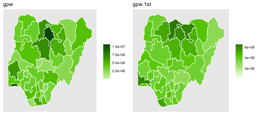
As can be seen in the summary, the package not only
merged the layer gpw to states, but also
generated its value per area of the target polygon and first- and
second-order spatial lag values for each. For inputs of type
RasterLayer, values per area are always also returned.
Whether or not spatial lags should be calculated can be controlled by
the optional Boolean argument spat.lag.
output = geomerge(gpw,na.rm=TRUE,target=states,
                  spat.lag=FALSE,silent=TRUE)
summary (output)
## geomerge completed: 1 datasets successfully integrated - run in static mode.
##
## The following 1 numerical variable(s) are available:
## gpwplot(output)
As in the case of Polygon data, the defaults of
geomerge have built-in implicit assumptions regarding zonal
statistics. The default zonal function is summation
(zonal.fun = sum). The package also supports all zonal
statistics consistent with the extract function in the
raster package.
output = geomerge(gpw,na.rm=TRUE,target=states,
                  spat.lag=FALSE,zonal.fun=min,silent=TRUE)
summary (output)
## geomerge completed: 1 datasets successfully integrated - run in static mode.
##
## The following 1 numerical variable(s) are available:
## gpwplot(output)
In geomerge, integration of point data
supports two different heuristics, which the user specifies via
point.agg. The first heuristic
(point.agg = "cnt") counts the occurrence of points in a
given unit of target. The second heuristic users
(point.agg = "sum") sums the values for all points in a
given unit. This heuristic is only appropriate for numeric
variables.
To illustrate, we use information on the conflict fatalities as
recorded in ACLED and the financial commitments of
development aid projects as recorded in AidData. We start
by looking at the event counts and the number of projects in each Local
Government Area of Nigeria throughout 2011 using
point.agg = "cnt". Then we examine the total umbers of
conflict fatalities and aid dollar commitments associated with those
areas.
# Run geomerge using point.agg = 'cnt
output = geomerge(ACLED$FATALITIES,AidData$commitme_1,
                  target=states,point.agg='cnt',silent=TRUE)
summary(output)
## geomerge completed: 2 datasets successfully integrated - run in static mode.
##
## The following 2 numerical variable(s) are available:
## ACLED.FATALITIES, AidData.commitme_1
##
## First and second order spatial lag values available.plot(output)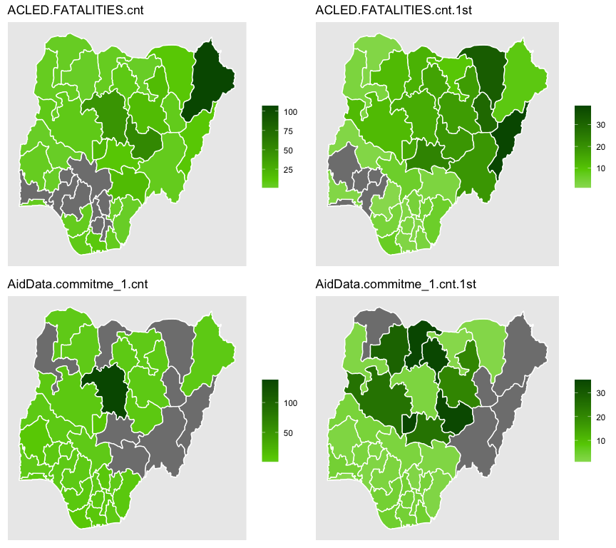
# Run geomerge using point.agg = 'sum
output = geomerge(ACLED$FATALITIES,AidData$commitme_1,
                  target=states,point.agg='sum',silent=TRUE)
summary(output)
## geomerge completed: 2 datasets successfully integrated - run in static mode.
##
## The following 2 numerical variable(s) are available:
## ACLED.FATALITIES, AidData.commitme_1
##
## First and second order spatial lag values available.plot(output)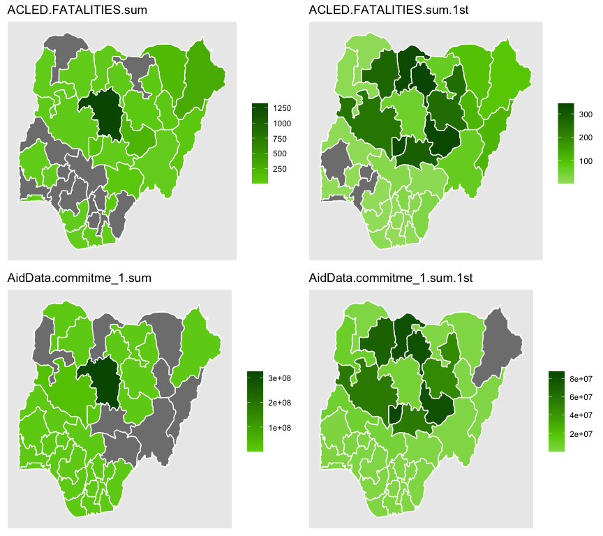
Dynamic integration of point data follows the same
process as before, but separated in a series of temporal units, thereby
generating a spatial panel. In geomerge, the temporal units
are specified through the time argument. The package
performs static integration if time = NA. For dynamic
integration, the user must specify
time = c(start_date, end_date, interval_length). All three
inputs must be strings, where interval_length
is defined in multiples of t_unit. The default value is
t_unit = "days". The package also accepts inputs of “secs”,
“mins”, “hours”, “months” or “years”.
In the following illustration, we employ the same data as before, but now include the “timestamp” column from both datasets. Information capturing the timing of observations is a prerequisite for dynamic integration. The information does not have to be at any specific level of precision, but does have to concern timing. We iterate through the whole year 2011 in one-month steps. In other words, we generate a county-month spatial panel.
# Run geomerge using point.agg = 'cnt
output = geomerge(ACLED$FATALITIES,AidData$commitme_1,
                  target=states,time=c("2011-01-01","2011-12-31","1"),
                  t_unit='months',point.agg='cnt',silent=TRUE)
summary(output)
## geomerge completed: 2 datasets successfully integrated - run in dynamic mode, spatial panel was generated.
##
## The following 2 numerical variable(s) are available:
## ACLED.FATALITIES, AidData.commitme_1
##
## First and second order spatial lag values available.
## First and second order temporal lag values available.plot(output)## Output data is spatial panel, showing results only for the last period. Use optional argument "period" to select specific time period.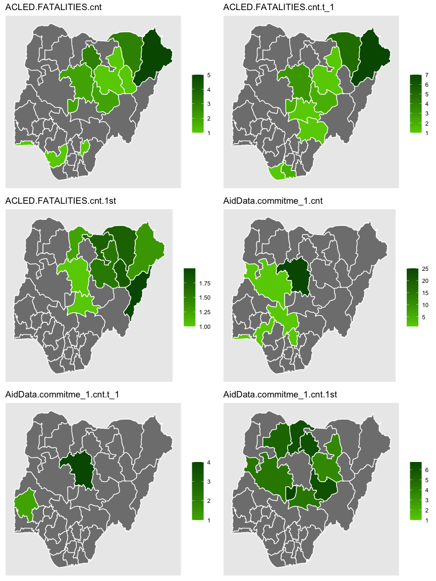
# Run geomerge using point.agg = 'cnt
output = geomerge(ACLED$FATALITIES,AidData$commitme_1,
                  target=states,time=c("2011-01-01","2011-12-31","1"),
                  t_unit='months',point.agg='sum',silent=TRUE)
summary(output)
## geomerge completed: 2 datasets successfully integrated - run in dynamic mode, spatial panel was generated.
##
## The following 2 numerical variable(s) are available:
## ACLED.FATALITIES, AidData.commitme_1
##
## First and second order spatial lag values available.
## First and second order temporal lag values available.plot(output)## Output data is spatial panel, showing results only for the last period. Use optional argument "period" to select specific time period.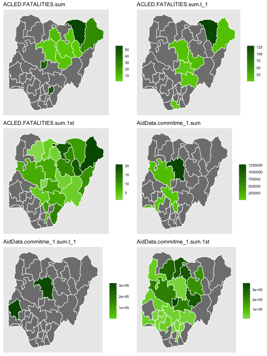
Note: By default, plot selects the last time period for
purposes of the visualization. If the user wishes to visualize any other
period, simply add the optional argument period to the
function. Also, first- and second-order time-lagged variables are
returned by default. The optional Boolean argument time.lag
controls this feature.
output = geomerge(ACLED$FATALITIES,AidData$commitme_1,
                  target=states,time=c("2011-01-01","2011-12-31","1"),
                  t_unit='months',point.agg='sum',time.lag=FALSE,silent=TRUE)
summary(output)
## geomerge completed: 2 datasets successfully integrated - run in dynamic mode, spatial panel was generated.
##
## The following 2 numerical variable(s) are available:
## ACLED.FATALITIES, AidData.commitme_1
##
## First and second order spatial lag values available.plot(output, period=3)## Output data is spatial panel, showing variables only for period 3, as specified.
Thus far, we have only considered integration targets in the form of
the Nigeria county polygons states. The
generateGrid function in geomerge allows the
user to easily generate a matching grid of a chosen resolution. For many
econometric applications, this option can be very useful.
# install.packages("sp")
require(sp)
## Loading required package: sp# Generate grid with 10 km cell size (input in m) in local CRS for Nigeria
states.grid <- generateGrid(states,
size= 10000, # meters
local.CRS=CRS("+init=epsg:26391"),
silent = TRUE)
# Run simple static integration with this grid as target
output = geomerge(ACLED$FATALITIES,target=states.grid,
point.agg='sum',silent=TRUE)
summary(output)## geomerge completed: 1 datasets successfully integrated - run in static mode.
##
## The following 1 numerical variable(s) are available:
## ACLED.FATALITIES
##
## First and second order spatial lag values available.plot(output)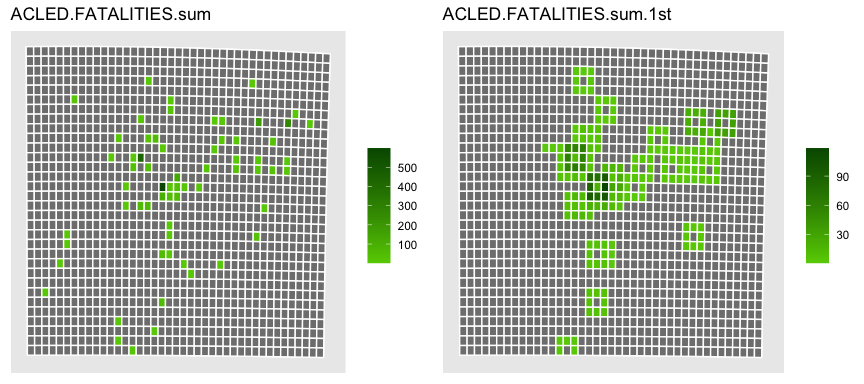
geomerge in R using
citation(package = 'geomerge')