
![]()
![]()
![]()
A Hilbert curve (also known as a Hilbert space-filling curve) is a continuous fractal space-filling curve first described by the German mathematician David Hilbert in 1891, as a variant of the space-filling Peano curves discovered by Giuseppe Peano in 1890 (from Wikipedia).
This package provides an easy access to using Hilbert curves in
ggplot2.
You can install the released version of gghilbertstrings from CRAN with:
install.packages("gghilbertstrings")You can install the development version from GitHub with:
# install.packages("remotes") # run only if not installed
remotes::install_github("Sumidu/gghilbertstrings")The gghilbertstrings package comes with functions for
fast plotting of Hilbert curves in ggplot. At it’s core is a fast RCpp
implementation that maps a 1D vector to a 2D position.
The gghilbertplot function creates a Hilbert curve and
plots individual data points to the corners of this plot. It
automatically rescales the used ID-variable to the full
range of the Hilbert curve. The method also automatically picks a
suitable level of detail able to represent all values of
ID.
The following figure shows different hilbert curves for different
maximum IDs.

The most simple way to plot data is to generate an id
column that ranges from 1 to n, where n is the largest value to use in
the Hilbert curve. Beware: The ids are rounded to
integers.
library(gghilbertstrings)

# val is the ID column used here
df <- tibble(val = 1:256,
       size = runif(256, 1, 5),        # create random sizes
       color = rep(c(1,2,3,4),64))     # create random colours

gghilbertplot(df, val,
                color = factor(color), # render color as a factor
                size = size,
                add_curve = T)         # also render the curves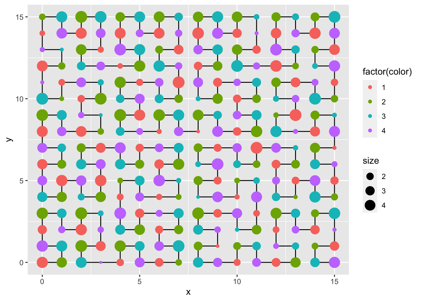
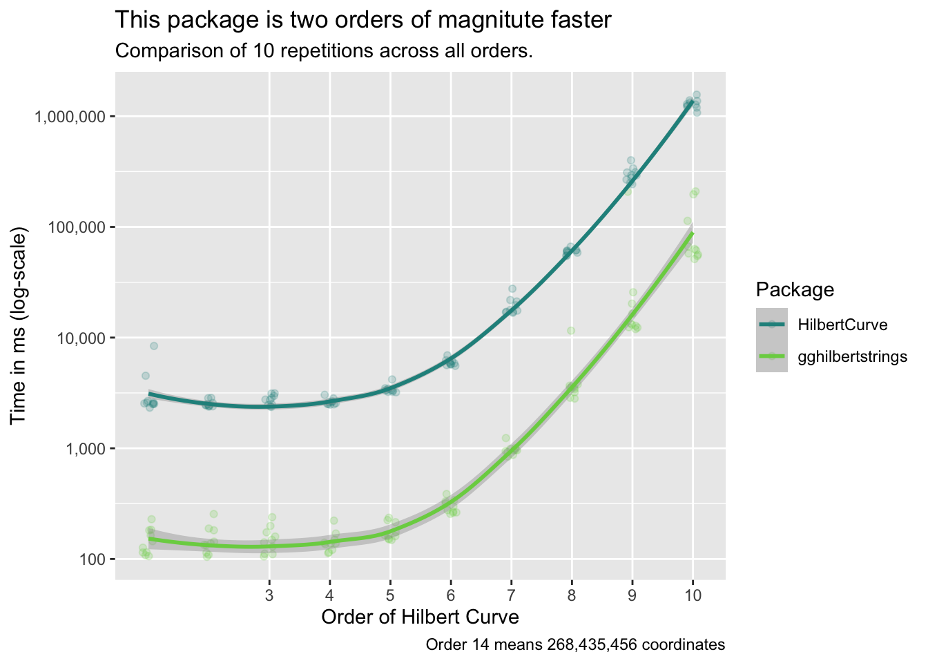
We run the creation of a coordinate system 10 times. This means creating 1 entry for every possible corner in the Hilbert Curve.
library(microbenchmark)
library(HilbertCurve)
library(tidyverse)
library(gghilbertstrings)
mb <- list()
for (i in 1:10) {
  df <- tibble(val = 1:4^i,
               size = runif(4^i, 1, 5),
               # create random sizes
               color = rep(c(1, 2, 3, 4), 4^(i - 1)))
  values <- df$val
  mb[[i]] <- microbenchmark(times = reps,
                     HilbertCurve = {
                       hc <- HilbertCurve(1, 4^i, level = i, newpage = FALSE)
                     },
                     gghilbertstrings = {
                       ggh <- hilbertd2xy(n = 4^i, values)
                     })
}
We use the
eliasdabbas/search-engine-results-flights-tickets-keywords
data set on Kaggle
as an example for a simple analysis. We map the full search URLs to the
Hilbert curve and then add points when the URL was present for a
specific search term. By comparing resulting facets we can see
systematic difference in which provides show up for which search
term.
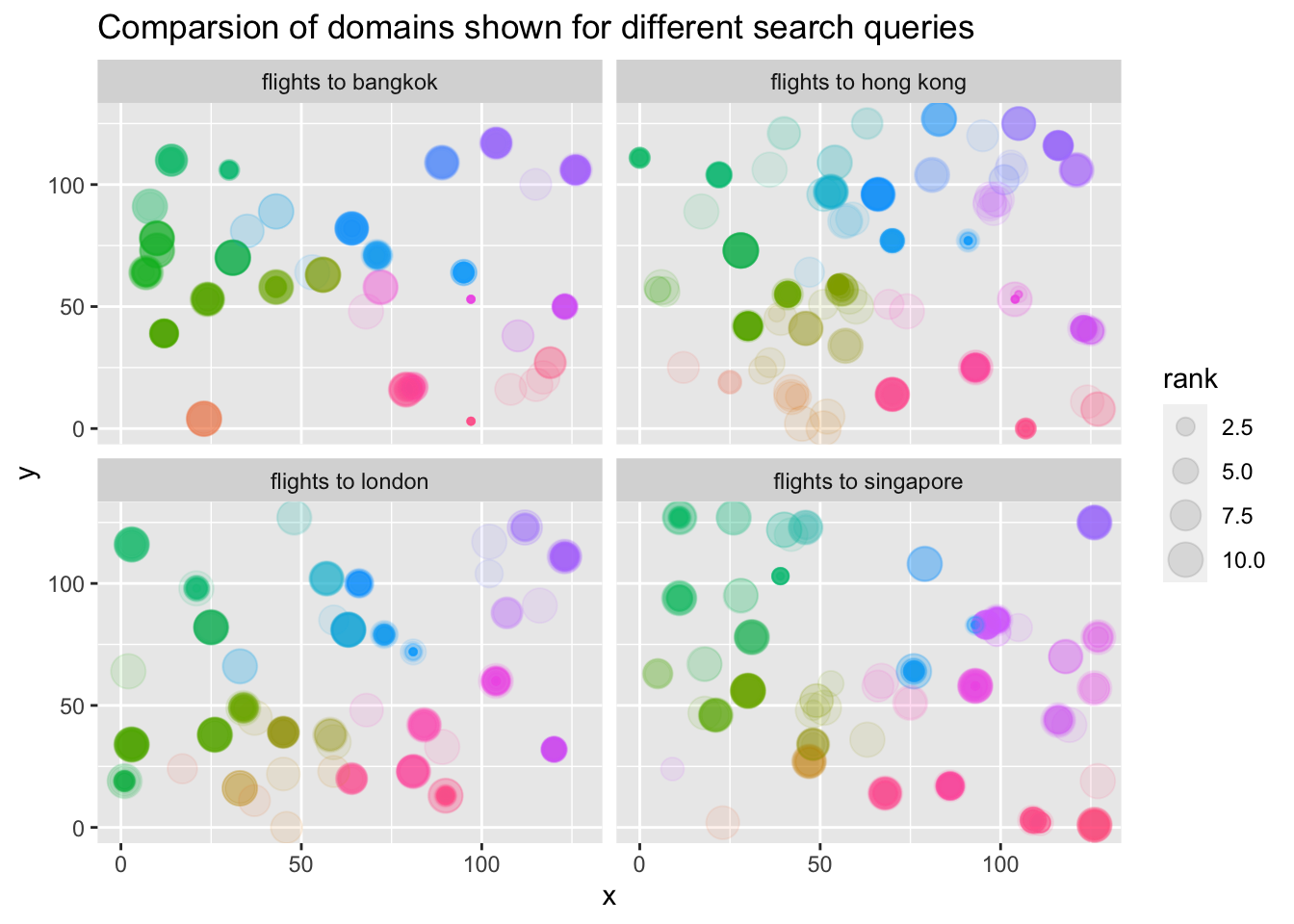
Link: https://www.kaggle.com/eliasdabbas/search-engine-results-flights-tickets-keywords under License CC0