![]()
![]()
![]()

The glottospace package facilitates the geospatial analysis of linguistic and cultural data. The aim of this package is to provide a streamlined workflow for working with spatio-linguistic data, including data import, cleaning, exploration, visualization and export. For example, with glottospace you can quickly match your own linguistic data to a location and plot it on a map. You can also calculate distances between languages based on their location or linguistic features and visualize those distances. In addition, with glottospace you can easily access global databases such as glottolog, WALS and D-PLACE from R and integrate them with your own data.
We’re still actively developing the glottospace package by adding new functions and improving existing ones. Although the package is stable, you might find bugs or encounter things you might find confusing. You can help us to improve the package by:
We’re currently writing a paper about the package presenting its full functionality. If you find the glottospace package useful, please cite it in your work:
#>
#> To cite glottospace in publications use:
#>
#>   Norder, S.J. et al. (2022). glottospace: R package for the geospatial
#>   analysis of linguistic and cultural data. URL
#>   https://github.com/SietzeN/glottospace.
#>
#> A BibTeX entry for LaTeX users is
#>
#>   @Unpublished{,
#>     title = {glottospace: R package for the geospatial analysis of linguistic and cultural data},
#>     author = {Sietze Norder},
#>     note = {Manuscript under preparation},
#>     url = {https://github.com/SietzeN/glottospace},
#>   }
The package uses two global databases: glottolog and WALS. In addition, glottospace builds on a combination of spatial and non-spatial packages, including sf, terra, tmap, mapview, rnaturalearth, and dplyr. If you use glottospace in one of your publications, please cite these data sources and packages as well.
You can install the latest release of glottospace from CRAN with:
# install.packages("glottospace")You can install the development version of glottospace from GitHub with:
# install.packages("devtools")
# devtools::install_github("SietzeN/glottospace", INSTALL_opts=c("--no-multiarch"))Before describing the functionality of glottospace, we give a quick demonstration of a typical workflow.
Imagine you’re working with languages in a particular region, and want to visualize them on a map. With glottospace this is easy! You could for example filter all languages in South America, and show which ones of them are isolate languages:
library(glottospace)

## Plot point data:
glottomap(continent = "South America", color = "isolate")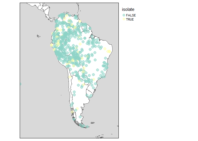
Languages are often represented with points, while in reality the speakers of a language can inhabit vast areas. glottospace works with point and polygon data. When polygon data is not available, you can interpolate the points and plot those.
## Filter by continent
glottopoints <- glottofilter(continent = "South America")
# Interpolate points to polygons:
glottopols <- glottospace(glottopoints, method = "voronoi")
# Plot polygon data:
glottomap(glottodata = glottopols, color = "family_size_rank")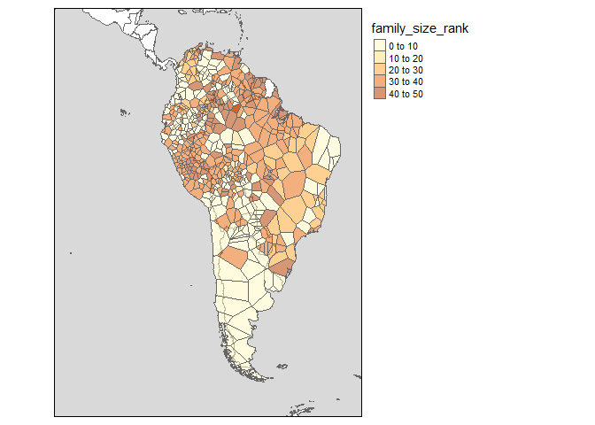
The glottospace package offers a wide range of functions to work with spatio-linguistic data. The functions are organized into the following function families, of which the core function generally has the same name as the family to which it belongs:
glottoget: download glottodata from remote server, or load locally stored glottodata.
glottocreate: create empty glottodata structure, to add data manually.
glottocheck: run interactive quality checks of user-provided glottodata.
glottoclean: clean-up glottodata.
glottojoin: join user-provided glottodata with other (often online) datasets.
glottosearch: search glottolog database for languages, language families, glottocodes, etc.
glottofilter: filter/subset glottodata based on linguistic and geographic features/variables.
glottodist: calculate differences/similarities between languages based on their features (linguistic, cultural, environmental, geographic, etc.).
glottoplot: visualizing differences/similarities between languages.
glottospace: make glottodata spatial, add coordinates, add spatial points or polygons to languages.
glottomap: visualize linguistic and cultural data on a map.
glottosave: save output generated by glottospace (data, figures, maps, etc.).
You can load locally stored glottodata (for example from an excel file or shapefile). The glottospace package has two built-in artificial demo datasets (“demodata” and “demosubdata”).
glottodata <- glottoget("demodata")
head(glottodata)
#>   glottocode var001 var002 var003
#> 1   yucu1253      Y      a      N
#> 2   tani1257   <NA>      b      Y
#> 3   ticu1245      Y      a      Y
#> 4   orej1242      N      b      N
#> 5   nade1244      N      c      Y
#> 6   mara1409      N      a      N
You can also load glottodata from online databases such as glottolog. You can download a raw version of the data (‘glottolog’), or an enriched/boosted version (‘glottobase’):
# To load glottobase:
glottobase <- glottoget("glottobase")
colnames(glottobase)
#>  [1] "glottocode"       "name"             "macroarea"        "isocode"
#>  [5] "countries"        "family_id"        "classification"   "parent_id"
#>  [9] "family"           "isolate"          "family_size"      "family_size_rank"
#> [13] "country" "continent" "sovereignty" "geometry"You can generate empty data structures that help you to add your own data in a structured way. These data structures can be saved to your local folder by specifying a filename (not demonstrated here).
glottocreate(glottocodes = c("yucu1253", "tani1257"), variables = 3, meta = FALSE)
#>   glottocode var001 var002 var003
#> 1   yucu1253     NA     NA     NA
#> 2   tani1257     NA     NA     NA
We’ve specified meta = FALSE, to indicate that we want to generate a ‘flat’ glottodata table. However, when creating glottodata, by default, several meta tables are included:
glottodata_meta <- glottocreate(glottocodes = c("yucu1253", "tani1257"), variables = 3)
summary(glottodata_meta)
#>              Length Class      Mode
#> glottodata    4     data.frame list
#> structure     6     data.frame list
#> description  11     data.frame list
#> references    9     data.frame list
#> remarks       5     data.frame list
#> contributors  5     data.frame list
#> sample        1     data.frame list
#> readme        2     data.frame list
#> lookup        2     data.frame list
The majority of these meta tables are added for the convenience of the user. The ‘structure’ table is the only one that is required for some of the functions in the glottospace package. A structure table can also be added later:
glottocreate_structuretable(varnames = c("var001", "var002", "var003"))
#>   varname type levels weight groups subgroups
#> 1  var001   NA     NA      1     NA        NA
#> 2  var002   NA     NA      1     NA        NA
#> 3  var003   NA     NA      1     NA        NA
More complex glottodata structures can also be generated. For example, in cases where you want to distinguish between groups within each language.
# Instead of creating a single table for all languages, you might want to create a list of tables (one table for each language)
glottocreate(glottocodes = c("yucu1253", "tani1257"),
                     variables = 3, groups = c("a", "b"), n = 2, meta = FALSE)
#> $yucu1253
#>     glottosubcode var001 var002 var003
#> 1 yucu1253_a_0001     NA     NA     NA
#> 2 yucu1253_a_0002     NA     NA     NA
#> 3 yucu1253_b_0001     NA     NA     NA
#> 4 yucu1253_b_0002     NA     NA     NA
#>
#> $tani1257
#>     glottosubcode var001 var002 var003
#> 1 tani1257_a_0001     NA     NA     NA
#> 2 tani1257_a_0002     NA     NA     NA
#> 3 tani1257_b_0001     NA     NA     NA
#> 4 tani1257_b_0002 NA NA NAIf you have your own data, you might want to do some interactive quality checks:
glottodata <- glottoget("demodata")
glottocheck(glottodata, diagnostic = FALSE)
#> No missing IDs
#> No duplicate IDs.
#> All variables have two or more levels (excluding NA)
#> Checking 6 glottocodes...
#> All IDs are valid glottocodes
#> Some columns have missing data.
#> Some rows have missing data.
We’ve now specified diagnostic = FALSE, but the default is to show some more extensive diagnostics (like a data coverage plot).
You can also check the metadata:
glottodata <- glottoget(glottodata = "demodata", meta = TRUE)
glottocheck(glottodata, checkmeta = TRUE)
#> No missing IDs
#> No duplicate IDs.
#> All variables have two or more levels (excluding NA)
#> Checking 6 glottocodes...
#> All IDs are valid glottocodes
#> Some columns have missing data.
#>       var001
#> count      1
#> Some rows have missing data.
#>          count
#> tani1257     1
#> This glottodataset contains the folowing tables: glottodata, structure, description, references, remarks, contributors, sample, readme, lookup
#> All types recognized
#> All weights are specified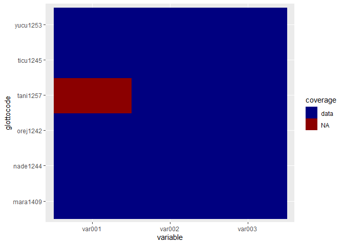
Once you’ve loaded glottodata, you might encounter some inconsistencies. For example, data-contributors might not have used a standardized way of coding missing values.
glottodata <- glottoget(glottodata = "demodata", meta = TRUE)
glottodata$structure
#>   varname   type levels weight groups subgroups
#> 1  var001   symm     NA      1     NA        NA
#> 2  var002 factor     NA      1     NA        NA
#> 3  var003   symm     NA      1     NA        NA
# glottodata <- glottoclean(glottodata)Join user-provided glottodata with other datasets, or with online databases.
# Join with glottospace
glottodata <- glottoget("demodata")
glottodatabase <- glottojoin(glottodata, with = "glottobase")
glottodataspace <- glottojoin(glottodata, with = "glottospace")

# Join a list of glottodata tables into a single table
glottodatalist <- glottocreate(glottocodes = c("yucu1253", "tani1257"),
                                       variables = 3, groups = c("a", "b"), n = 2, meta = FALSE)
glottodatatable <- glottojoin(glottodata = glottodatalist)As demonstrated in the example above, you can search glottodata for a specific search term
You can search for a match in all columns:
glottosearch(search = "yurakar")
#> Simple feature collection with 1 feature and 15 fields
#> Geometry type: POINT
#> Dimension:     XY
#> Bounding box:  xmin: -65.1224 ymin: -16.7479 xmax: -65.1224 ymax: -16.7479
#> Geodetic CRS:  WGS 84
#>      glottocode     name     macroarea isocode countries family_id
#> 7546   yura1255 Yuracaré South America     yuz        BO  yura1255
#>      classification parent_id   family isolate family_size family_size_rank
#> 7546           <NA>      <NA> Yuracaré    TRUE           1                1
#>      country     continent sovereignty                  geometry
#> 7546 Bolivia South America     Bolivia POINT (-65.1224 -16.7479)
Or limit the search to specific columns:
glottosearch(search = "Yucuni", columns = c("name", "family"))
#> Simple feature collection with 2 features and 15 fields
#> Geometry type: POINT
#> Dimension:     XY
#> Bounding box:  xmin: -97.91818 ymin: -0.76075 xmax: -71.0033 ymax: 17.23743
#> Geodetic CRS:  WGS 84
#>      glottocode              name     macroarea isocode countries family_id
#> 7532   yucu1253            Yucuna South America     ycn  BR;CO;PE  araw1281
#> 7533   yucu1254 Yucunicoco Mixtec North America                MX  otom1299
#>                                                      classification parent_id
#> 7532                            araw1281/japu1236/nucl1764/yucu1252  yucu1252
#> 7533 otom1299/east2557/amuz1253/mixt1422/mixt1423/mixt1427/sout3179  sout3179
#>           family isolate family_size family_size_rank  country     continent
#> 7532    Arawakan   FALSE          77               40 Colombia South America
#> 7533 Otomanguean   FALSE         182               44   Mexico North America
#>      sovereignty                   geometry
#> 7532    Colombia  POINT (-71.0033 -0.76075)
#> 7533      Mexico POINT (-97.91818 17.23743)
Sometimes you don’t find a match:
glottosearch(search = "matsigenka")[,"name"]
#> Simple feature collection with 0 features and 1 field
#> Bounding box:  xmin: NA ymin: NA xmax: NA ymax: NA
#> Geodetic CRS:  WGS 84
#> [1] name     geometry
#> <0 rows> (or 0-length row.names)
If you can’t find what you’re looking for, you can increase the tolerance:
glottosearch(search = "matsigenka", tolerance = 0.2)[,"name"]
#> Simple feature collection with 1 feature and 1 field
#> Geometry type: POINT
#> Dimension:     XY
#> Bounding box:  xmin: -74.4371 ymin: -11.5349 xmax: -74.4371 ymax: -11.5349
#> Geodetic CRS:  WGS 84
#>               name                  geometry
#> 4779 Nomatsiguenga POINT (-74.4371 -11.5349)
Aha! There it is: ‘Machiguenga’
glottosearch(search = "matsigenka", tolerance = 0.4)[,"name"]
#> Simple feature collection with 12 features and 1 field
#> Geometry type: POINT
#> Dimension:     XY
#> Bounding box:  xmin: -74.4371 ymin: -14.9959 xmax: 166.738 ymax: 13.5677
#> Geodetic CRS:  WGS 84
#> First 10 features:
#>                    name                   geometry
#> 1708 Eastern Maninkakan   POINT (-10.5394 9.33048)
#> 3061    Kita Maninkakan   POINT (-9.49151 13.1798)
#> 3145   Konyanka Maninka   POINT (-8.89972 8.04788)
#> 3724   Maasina Fulfulde   POINT (-3.64763 11.1324)
#> 3740        Machiguenga  POINT (-72.5017 -12.1291)
#> 3894           Mandinka POINT (-15.65395 12.81652)
#> 3930          Mansoanka   POINT (-15.9202 12.8218)
#> 4033  Matigsalug Manobo     POINT (125.16 7.72124)
#> 4779      Nomatsiguenga  POINT (-74.4371 -11.5349)
#> 5371 Piamatsina POINT (166.738 -14.9959)filter, select, query
eurasia <- glottofilter(continent = c("Europe", "Asia"))
wari <- glottofilter(glottodata = glottodata, glottocode = "wari1268")
#> No search results. You might consider using glottosearch() first
indo_european <- glottofilter(glottodata = glottodata, family = 'Indo-European')
south_america <- glottofilter(glottodata = glottodata, continent = "South America")
colovenz <- glottofilter(country = c("Colombia", "Venezuela"))
# arawtuca <- glottofilter(glottodata = glottodata, expression = family %in% c("Arawakan", "Tucanoan"))Quantify differences and similarities between languages glottodistances: calculating similarities between languages based on linguistic/cultural features
# In order to be able to calculate linguistic distances a structure table is required, that's why we specify meta = TRUE.
glottodata <- glottoget("demodata", meta = TRUE)
glottodist <- glottodist(glottodata = glottodata)
#> glottocode used as id
#> Values in binary columns (symm/asymm) recoded to TRUE/FALSE
#> Missing values recoded to NA

# As we've seen above, in case you have glottodata without a structure table, you can add it:
glottodata <- glottoget("demodata", meta = FALSE)
structure <- glottocreate_structuretable()
glottodata <- glottocreate_addtable(glottodata, structure, name = "structure")Visualizing differences (distances) between languages based on linguistic, cultural, and environmental features.
glottodata <- glottoget("demodata", meta = TRUE)
glottodist <- glottodist(glottodata = glottodata)
#> glottocode used as id
#> Values in binary columns (symm/asymm) recoded to TRUE/FALSE
#> Missing values recoded to NA
glottoplot(glottodist = glottodist)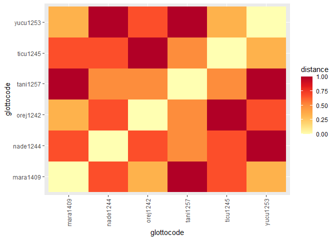
This family of functions turns glottodata into a spatial object. As we’ve illustrated above, these can be either glottopoints or glottopols
glottodata <- glottoget("demodata")
glottospacedata <- glottospace(glottodata, method = "buffer", radius = 5)
#> Buffer created with a radius of 5 km.
# By default, the projection of maps is equal area, and shape is not preserved:
glottomap(glottospacedata)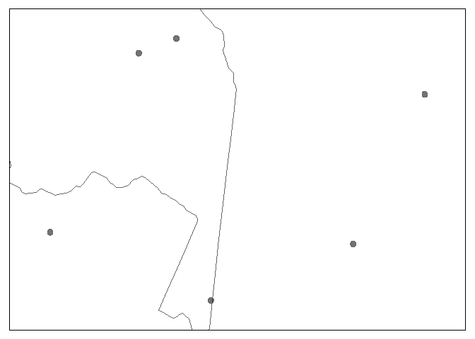
With glottomap you can quickly visualize the location of languages. Below we show simple static maps, but you can also create dynamic maps by specifying type = “dynamic”.
To select languages, you don’t need to call glottofilter() first, but you can use glottomap() directly. Behind the scenes glottomap() passes those arguments on to glottofilter().
glottomap(country = "Colombia")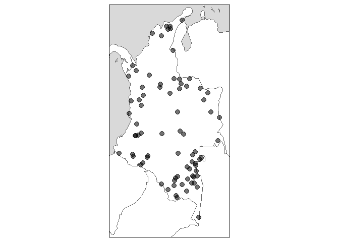
However, you can also create maps with other glottodata. For example, we might want to create a world map highlighting the largest language families
glottodata <- glottoget()
families <- dplyr::count(glottodata, family, sort = TRUE)

# highlight 10 largest families:
glottodata <- glottospotlight(glottodata = glottodata, spotcol = "family", spotlight = families$family[1:10], spotcontrast = "family", bgcontrast = "family")

# Create map
glottomap(glottodata, color = "color")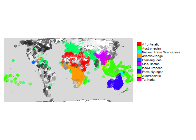
All output generated with the glottospace package (data, figures, maps, etc.) can be saved with a single command.
glottodata <- glottoget("demodata", meta = FALSE)
# Saves as .xlsx
# glottosave(glottodata, filename = "glottodata")

# Saves as .GPKG
glottospacedata <- glottospace(glottodata)
# glottosave(glottodata, filename = "glottodata")

# By default, static maps are saved as .png, dynamic maps are saved as .html
glottomap <- glottomap(glottodata)
# glottosave(glottomap, filename = "glottomap")