![]()
![]()
![]()

This package implements some graph layout algorithms that are not
available in igraph.
A detailed introductory tutorial for graphlayouts and ggraph can be found here.
The package implements the following algorithms:
# dev version
remotes::install_github("schochastics/graphlayouts")

# CRAN
install.packages("graphlayouts")This example is a bit of a special case since it exploits some weird issues in igraph.
library(igraph)
library(ggraph)
library(graphlayouts)

set.seed(666)
pa <- sample_pa(1000, 1, 1, directed = F)

ggraph(pa, layout = "nicely") +
    geom_edge_link0(width = 0.2, colour = "grey") +
    geom_node_point(col = "black", size = 0.3) +
    theme_graph()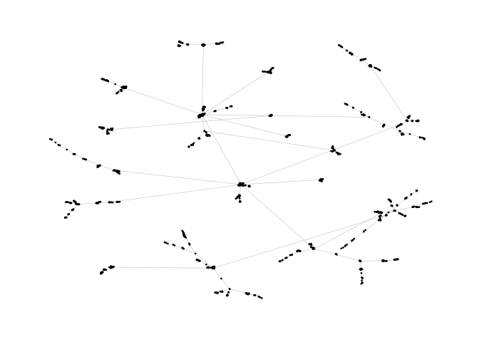
ggraph(pa, layout = "stress") +
    geom_edge_link0(width = 0.2, colour = "grey") +
    geom_node_point(col = "black", size = 0.3) +
    theme_graph()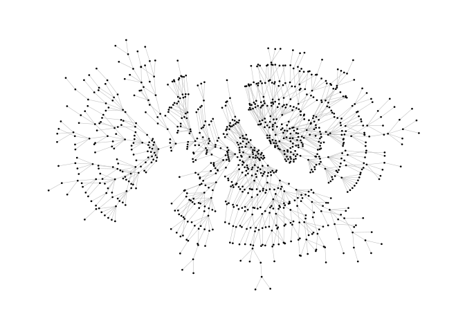
Stress majorization also works for networks with several components. It relies on a bin packing algorithm to efficiently put the components in a rectangle, rather than a circle.
set.seed(666)
g <- disjoint_union(
    sample_pa(10, directed = FALSE),
    sample_pa(20, directed = FALSE),
    sample_pa(30, directed = FALSE),
    sample_pa(40, directed = FALSE),
    sample_pa(50, directed = FALSE),
    sample_pa(60, directed = FALSE),
    sample_pa(80, directed = FALSE)
)

ggraph(g, layout = "nicely") +
    geom_edge_link0() +
    geom_node_point() +
    theme_graph()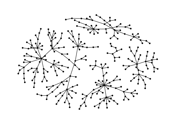
ggraph(g, layout = "stress", bbox = 40) +
    geom_edge_link0() +
    geom_node_point() +
    theme_graph()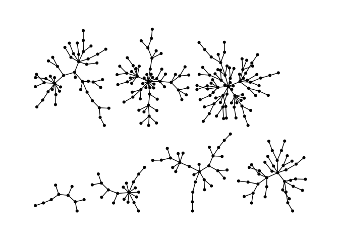
Backbone layouts are helpful for drawing hairballs.
set.seed(665)
# create network with a group structure
g <- sample_islands(9, 40, 0.4, 15)
g <- simplify(g)
V(g)$grp <- as.character(rep(1:9, each = 40))

ggraph(g, layout = "stress") +
    geom_edge_link0(colour = rgb(0, 0, 0, 0.5), width = 0.1) +
    geom_node_point(aes(col = grp)) +
    scale_color_brewer(palette = "Set1") +
    theme_graph() +
    theme(legend.position = "none")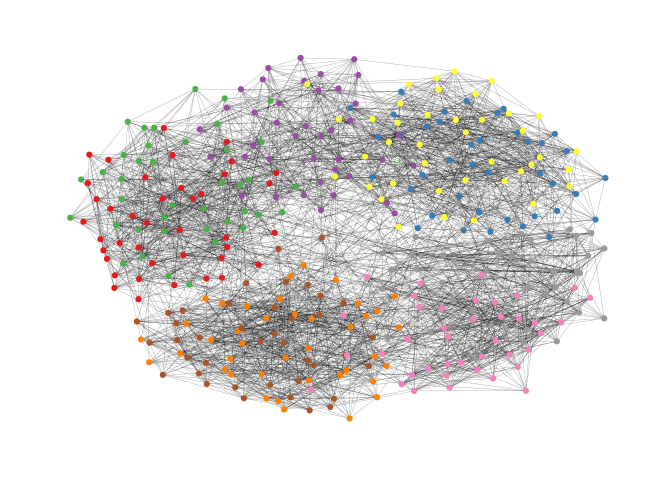
The backbone layout helps to uncover potential group structures based on edge embeddedness and puts more emphasis on this structure in the layout.
bb <- layout_as_backbone(g, keep = 0.4)
E(g)$col <- FALSE
E(g)$col[bb$backbone] <- TRUE

ggraph(g, layout = "manual", x = bb$xy[, 1], y = bb$xy[, 2]) +
    geom_edge_link0(aes(col = col), width = 0.1) +
    geom_node_point(aes(col = grp)) +
    scale_color_brewer(palette = "Set1") +
    scale_edge_color_manual(values = c(rgb(0, 0, 0, 0.3), rgb(0, 0, 0, 1))) +
    theme_graph() +
    theme(legend.position = "none")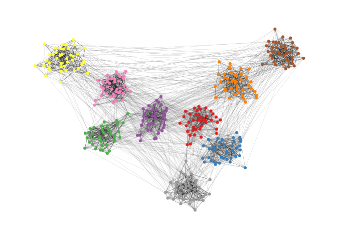
The function layout_with_focus() creates a radial layout
around a focal node. All nodes with the same distance from the focal
node are on the same circle.
library(igraphdata)
library(patchwork)
data("karate")

p1 <- ggraph(karate, layout = "focus", focus = 1) +
    draw_circle(use = "focus", max.circle = 3) +
    geom_edge_link0(edge_color = "black", edge_width = 0.3) +
    geom_node_point(aes(fill = as.factor(Faction)), size = 2, shape = 21) +
    scale_fill_manual(values = c("#8B2323", "#EEAD0E")) +
    theme_graph() +
    theme(legend.position = "none") +
    coord_fixed() +
    labs(title = "Focus on Mr. Hi")

p2 <- ggraph(karate, layout = "focus", focus = 34) +
    draw_circle(use = "focus", max.circle = 4) +
    geom_edge_link0(edge_color = "black", edge_width = 0.3) +
    geom_node_point(aes(fill = as.factor(Faction)), size = 2, shape = 21) +
    scale_fill_manual(values = c("#8B2323", "#EEAD0E")) +
    theme_graph() +
    theme(legend.position = "none") +
    coord_fixed() +
    labs(title = "Focus on John A.")

p1 + p2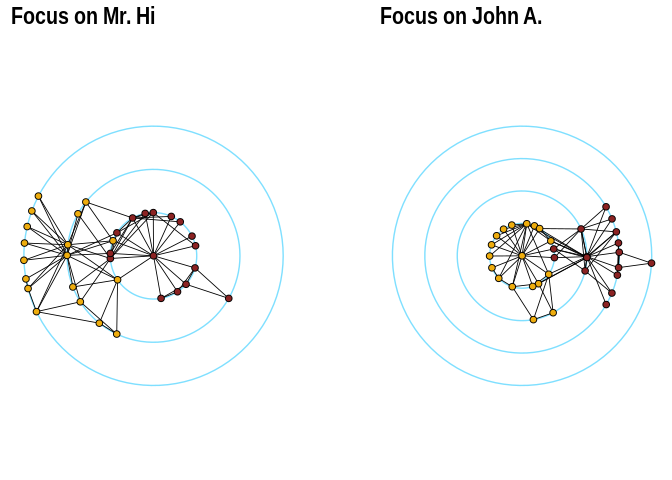
The function layout_with_centrality creates a radial
layout around the node with the highest centrality value. The further
outside a node is, the more peripheral it is.
library(igraphdata)
library(patchwork)
data("karate")

bc <- betweenness(karate)
p1 <- ggraph(karate, layout = "centrality", centrality = bc, tseq = seq(0, 1, 0.15)) +
    draw_circle(use = "cent") +
    annotate_circle(bc, format = "", pos = "bottom") +
    geom_edge_link0(edge_color = "black", edge_width = 0.3) +
    geom_node_point(aes(fill = as.factor(Faction)), size = 2, shape = 21) +
    scale_fill_manual(values = c("#8B2323", "#EEAD0E")) +
    theme_graph() +
    theme(legend.position = "none") +
    coord_fixed() +
    labs(title = "betweenness centrality")


cc <- closeness(karate)
p2 <- ggraph(karate, layout = "centrality", centrality = cc, tseq = seq(0, 1, 0.2)) +
    draw_circle(use = "cent") +
    annotate_circle(cc, format = "scientific", pos = "bottom") +
    geom_edge_link0(edge_color = "black", edge_width = 0.3) +
    geom_node_point(aes(fill = as.factor(Faction)), size = 2, shape = 21) +
    scale_fill_manual(values = c("#8B2323", "#EEAD0E")) +
    theme_graph() +
    theme(legend.position = "none") +
    coord_fixed() +
    labs(title = "closeness centrality")

p1 + p2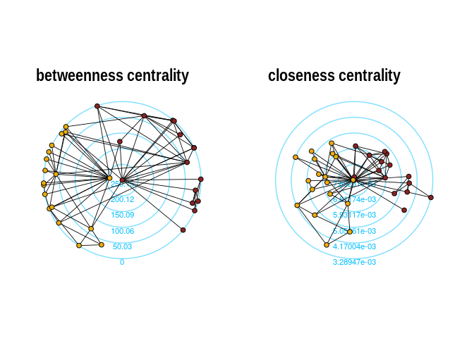
graphlayouts implements two algorithms for visualizing
large networks (<100k nodes). layout_with_pmds() is
similar to layout_with_mds() but performs the
multidimensional scaling only with a small number of pivot nodes.
Usually, 50-100 are enough to obtain similar results to the full
MDS.
layout_with_sparse_stress() performs stress majorization
only with a small number of pivots (~50-100). The runtime performance is
inferior to pivotMDS but the quality is far superior.
A comparison of runtimes and layout quality can be found in the wiki
tl;dr: both layout algorithms appear to be faster than
the fastest igraph algorithm layout_with_drl().
Below are two examples of layouts generated for large graphs using
layout_with_sparse_stress()
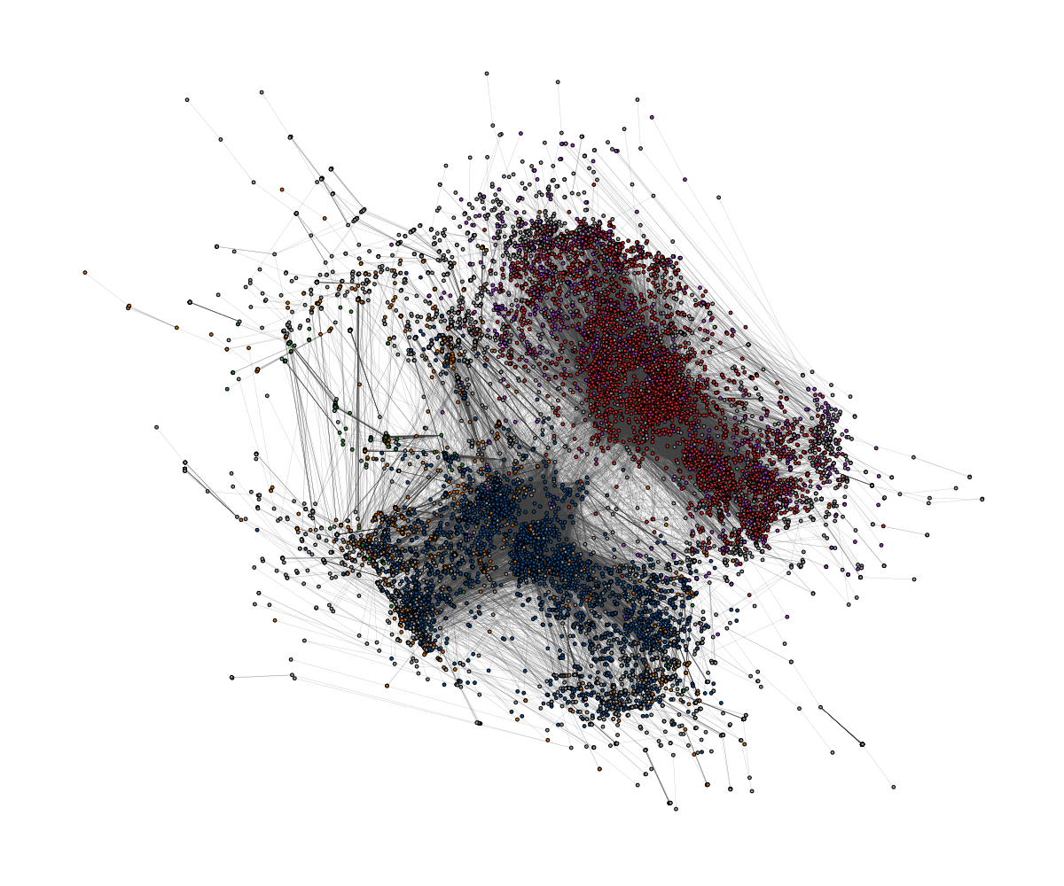 A retweet network with 18k nodes and 61k edges
 A network of football players with 165K nodes and 6M edges.
layout_as_dynamic() allows you to visualize snapshots of
longitudinal network data. Nodes are anchored with a reference layout
and only moved slightly in each wave depending on deleted/added edges.
In this way, it is easy to track down specific nodes throughout time.
Use patchwork to put the individual plots next to each
other.
# remotes::install_github("schochastics/networkdata")
library(networkdata)
# longitudinal dataset of friendships in a school class
data("s50")

xy <- layout_as_dynamic(s50, alpha = 0.2)
pList <- vector("list", length(s50))

for (i in seq_along(s50)) {
    pList[[i]] <- ggraph(s50[[i]], layout = "manual", x = xy[[i]][, 1], y = xy[[i]][, 2]) +
        geom_edge_link0(edge_width = 0.6, edge_colour = "grey66") +
        geom_node_point(shape = 21, aes(fill = as.factor(smoke)), size = 3) +
        geom_node_text(aes(label = 1:50), repel = T) +
        scale_fill_manual(
            values = c("forestgreen", "grey25", "firebrick"),
            labels = c("no", "occasional", "regular"),
            name = "smoking",
            guide = ifelse(i != 2, "none", "legend")
        ) +
        theme_graph() +
        theme(legend.position = "bottom") +
        labs(title = paste0("Wave ", i))
}
wrap_plots(pList)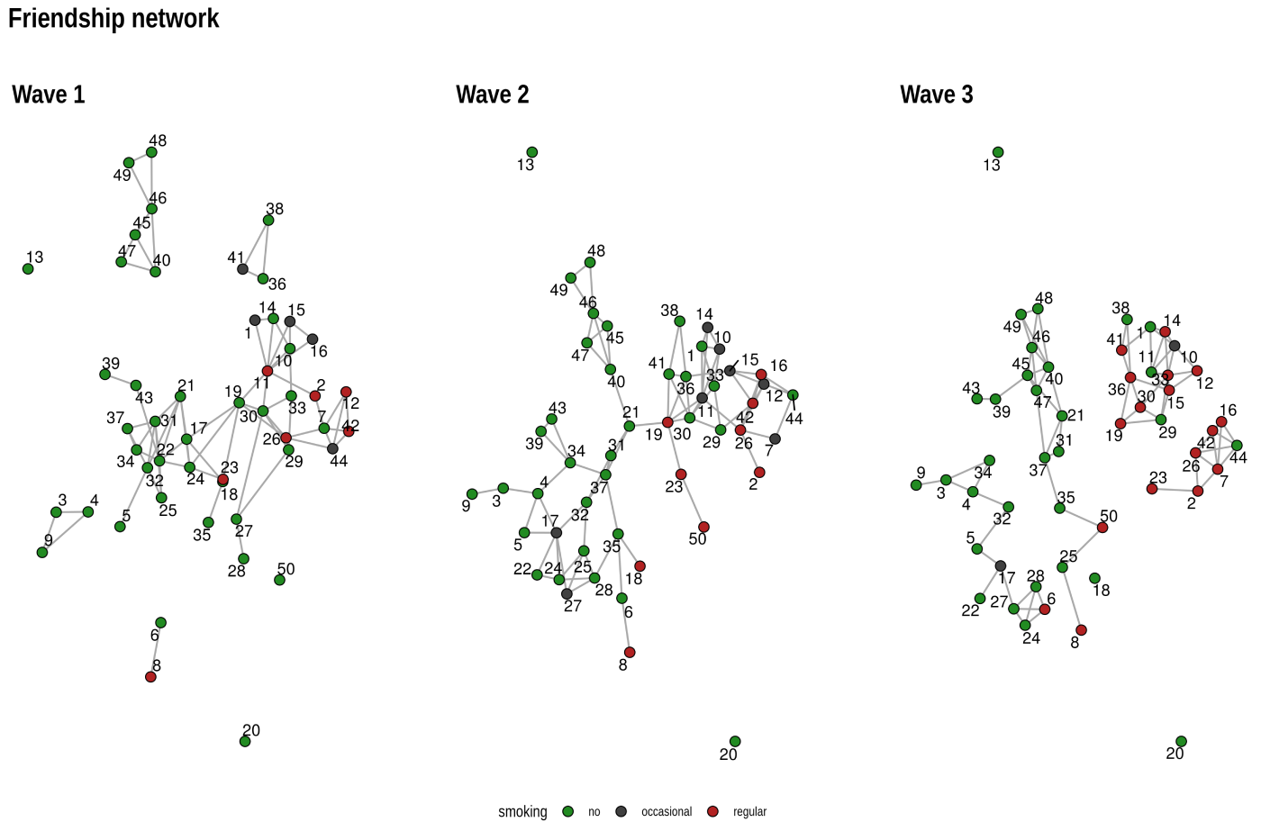
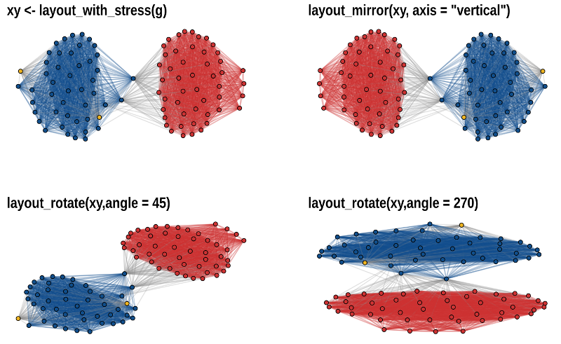
The functions layout_mirror() and
layout_rotate() can be used to manipulate an existing
layout
Simply open an issue on GitHub.
If you have an idea (but no code yet), open an issue on GitHub. If you want to contribute with a specific feature and have the code ready, fork the repository, add your code, and create a pull request.
The easiest way is to open an issue - this way, your question is also visible to others who may face similar problems.
Please note that the graphlayouts project is released with a Contributor Code of Conduct. By contributing to this project, you agree to abide by its terms.