The handwriter package performs writership analysis of a handwritten questioned document where the questioned document was written by one of closed-set of potential writers. For example, a handwritten bomb threat is found in a science classroom, and the police are able to determine that the note could only have been written by one of the students in 4th period science. The handwriter package builds a statistical model to estimate a writer profile from known handwriting samples from each writer in the closed-set. A writer profile is also estimated from the questioned document. The statistical model compares the writer profile from the questioned document with each of the writer profiles from the closed-set of potential writers and estimates the posterior probability that each closed-set writer wrote the questioned document.
You can install handwriter from CRAN with:
install.packages("handwriter")You can install the development version of handwriter from GitHub with:
# install.packages("devtools")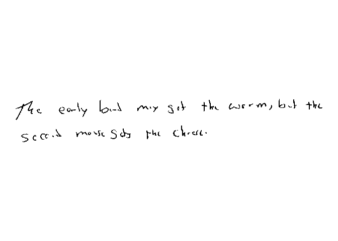
devtools::install_github("CSAFE-ISU/handwriter")The file “phrase_example.png” is a scanned PNG of handwriting from
the CSAFE Handwriting Database. This PNG image is included in the
handwriter package in a folder called “extdata.” Use the helper function
handwriter_example() to find the path to where
“phrase_example.png” is saved on your computer.
Use processDocument() to
library(handwriter)
phrase <- system.file("extdata", "phrase_example.png", package = "handwriter")
doc <- processDocument(phrase)
#> path in readPNGBinary: /private/var/folders/1z/jk9bqhdd06j1fxx0_xm2jj980000gn/T/RtmplsdN6z/temp_libpath947954bb6036/handwriter/extdata/phrase_example.png
#> Starting Processing...
#> Getting Nodes...
#> Skeletonizing writing...
#> Splitting document into components...
#> Merging nodes...
#> Finding paths...
#> Split paths into graphs...
#> Organizing graphs...
#> Creating graph lists...
#> Adding character features...
#> Document processing complete
We can view the image:
plotImage(doc)
We can view the thinned image:
plotImageThinned(doc)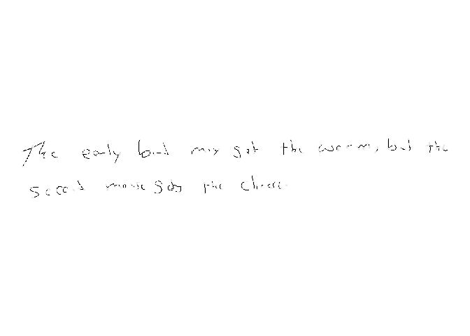
We can also view the nodes:
plotNodes(doc)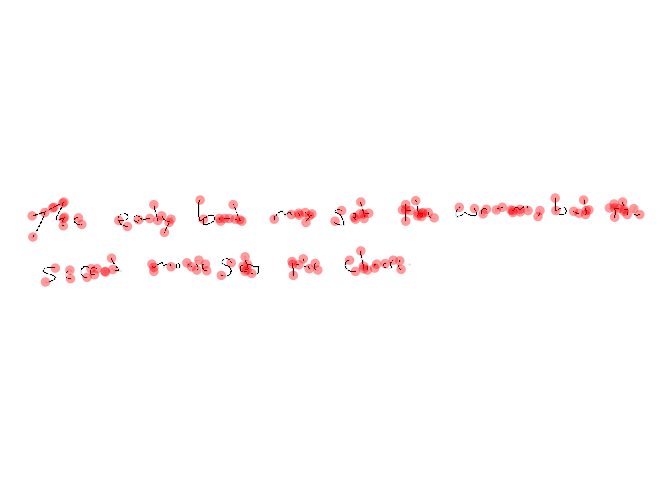
This section explains how to perform handwriting analysis on questioned documents using handwriter. In particular, handwriter addresses the scenario where an investigator has a questioned handwritten document, a group of persons of interest has been identified, and the questioned document had to have been written by one of the persons of interest. For example, imagine that a handwritten bomb threat was left at a office building’s main desk and the police discover that the note had to have been written by one of the one hundred employees working that day. More details on this method can be found in [Crawford 2022].
Create a new folder called main_dir on your computer to
hold the handwriting documents to be analyzed. When we create a new
clustering template and fit a statistical model, those files will also
be stored in this folder. Create a sub-folder in main_dir
called data. In the data folder, create
sub-folders called model_docs,
questioned_docs, and template_docs. The folder
structure will look like this:
├── main_dir
│   ├── data
│   │   ├── model_docs
│   │   ├── questioned_docs
│ │ ├── template_docsSave the handwritten documents that you want to use to train a new
cluster template as PNG images in
main_dir > data > template_docs. The template
training documents need to be from writers that are NOT people of
interest. Name all of the PNG images with a consistent format that
includes an ID for the writer. For example, the PNG images could be
named “writer0001.png”, “writer0002.png”, “writer0003.png” and so
on.
Next, create a new cluster template from the documents in
main_dir > data > template_docs with the function
make_clustering_template. This function
template_docs, decomposing the handwriting into component
shapes called graphs. The processed graphs are saved in RDS
files in main_dir \> data \> template_graphs.K starting cluster centers using seed
centers_seed for reproducibility.K starting cluster
centers and the selected graphs. The algorithm iteratively groups the
selected graphs into K clusters. The final grouping of
K clusters is the cluster template.writer_indices is a vector of the start and stop characters
of the writer ID in the PNG image file name. For example, if the PNG
images are named “writer0001.png”, “writer0002.png”, “writer0003.png”,
and so on, writer_indices = c(7,10)num_dist_cores.template <- make_clustering_template(
main_dir = "path/to/main_dir",
template_docs = "path/to/main_dir/data/template_docs",
writer_indices = c(7,10),
centers_seed = 100,
K = 40,
num_dist_cores = 4,
max_iters = 25)Type ?make_clustering_template in the RStudio console
for more information about the function’s arguments.
For the remainder of this tutorial, we use a small example cluster
template, example_cluster_template included in
handwriter.
template <- example_cluster_templateThe idea behind the cluster template and the hierarchical model is that we can decompose a handwritten document into component graphs, assign each graph to the nearest cluster, the cluster with the closest shape, in the cluster template, and count the number of graphs in each cluster. We characterize writers by the number of a writer’s graphs that are assigned to each cluster. We refer to this as a writer’s cluster fill counts and it serves as writer profile.
We can plot the cluster fill counts for each writer in the template training set. First we format the template data to get the cluster fill counts in the proper format for the plotting function.
template_data <- format_template_data(template = template)
plot_cluster_fill_counts(template_data, facet = TRUE)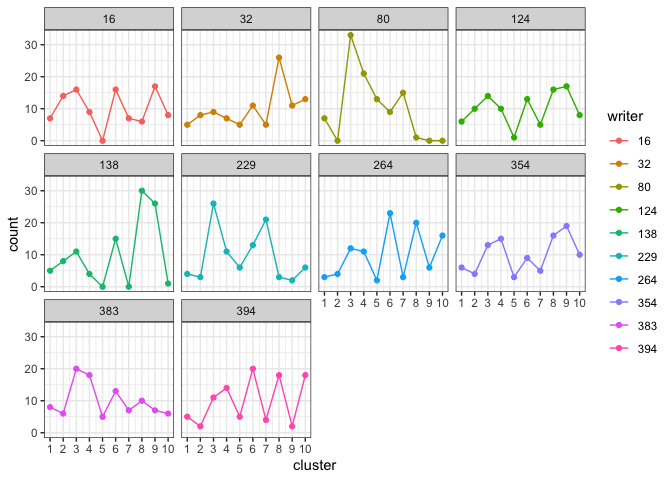
We will use handwriting samples from each person of interest, calculate the cluster fill counts from each sample using the cluster template, and fit a hierarchical model to estimate each person of interest’s true cluster fill counts.
Save your known handwriting samples from the persons of interest in
main_dir \> data \> model_docs as PNG images. The
model requires three handwriting samples from each person of interest.
Each sample should be at least one paragraph in length. Name the PNG
images with a consistent format so that all file names are the same
length and the writer ID’s are in the same location. For example,
“writer0001_doc1.png”, “writer0001_doc2.png”, “writer0001_doc3.png”,
“writer0002_doc1.png”, and so on.
We fit a hierarchical model with the function fit_model.
This function does the following:
model_docs,
decomposing the handwriting into component graphs. The processed graphs
are saved in RDS files in
main_dir \> data \> model_graphs.In this example, we use 4000 MCMC iterations for the model. The
inputs writer_indices and doc_indices are the
starting and stopping characters in the model training documents file
names that contains the writer ID and a document name.
model <- fit_model(main_dir = "path/to/main_dir",
                   model_docs = "path/to/main_dir/data/model_docs",
                   num_iters = 4000,
                   num_chains = 1,
                   num_cores = 2,
                   writer_indices = c(7, 10),
                   doc_indices = c(11, 14))
For this tutorial, we will use the small example model,
example_model, included in handwriter. This model was
trained from three documents each from writers 9, 30, 203, 238, and 400
from the CSAFE
handwriting database.
model <- example_modelWe can plot the cluster fill counts for each person of interest. (NOTE: We had to format the template data to work with the plotting function, but the model data is already in the correct format.)
plot_cluster_fill_counts(formatted_data=model, facet = TRUE)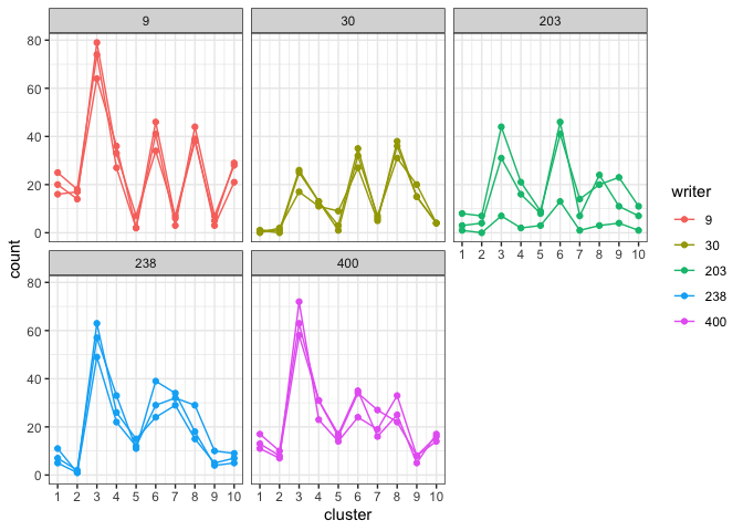 The bars across the top of each graph show the Writer ID. Each graph has
a line for each known handwriting sample from a given writer.
The bars across the top of each graph show the Writer ID. Each graph has
a line for each known handwriting sample from a given writer.
If you are interested in the variables used by the hierarchical model, continue reading this section. Otherwise, feel free to skip to the next section to learn how to analyze questioned documents.
We can list the variables in the model:
names(as.data.frame(coda::as.mcmc(model$fitted_model[[1]])))
#>  [1] "eta[1]"   "eta[2]"   "eta[3]"   "eta[4]"   "eta[5]"   "gamma[1]"
#>  [7] "gamma[2]" "gamma[3]" "gamma[4]" "gamma[5]" "mu[1,1]"  "mu[2,1]"
#> [13] "mu[3,1]"  "mu[1,2]"  "mu[2,2]"  "mu[3,2]"  "mu[1,3]"  "mu[2,3]"
#> [19] "mu[3,3]"  "mu[1,4]"  "mu[2,4]"  "mu[3,4]"  "mu[1,5]"  "mu[2,5]"
#> [25] "mu[3,5]"  "pi[1,1]"  "pi[2,1]"  "pi[3,1]"  "pi[1,2]"  "pi[2,2]"
#> [31] "pi[3,2]"  "pi[1,3]"  "pi[2,3]"  "pi[3,3]"  "pi[1,4]"  "pi[2,4]"
#> [37] "pi[3,4]"  "pi[1,5]"  "pi[2,5]"  "pi[3,5]"  "tau[1,1]" "tau[2,1]"
#> [43] "tau[3,1]" "tau[1,2]" "tau[2,2]" "tau[3,2]" "tau[1,3]" "tau[2,3]"
#> [49] "tau[3,3]" "tau[1,4]" "tau[2,4]" "tau[3,4]" "tau[1,5]" "tau[2,5]"
#> [55] "tau[3,5]"
View a description of a variable with the about_variable
function.
about_variable(variable = "mu[1,1]", model = model)
#> [1] "Mu is the location parameter of a wrapped-Cauchy distribution for writer ID w0009 and cluster 1"
View a trace plot of a variable.
plot_trace(variable = "mu[1,1]", model = model)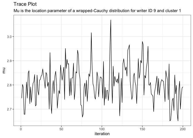
If we need to, we can drop the beginning MCMC iterations for burn-in. For example, if we want to drop the first 25 iterations, we use
model <- drop_burnin(model, burn_in = 25)If we want to save the updated model as the current model for this
project, replace model.rds in the data folder
with
saveRDS(model, file='data/model.rds')Save your questioned document(s) in
main_dir > data > questioned_docs as PNG images.
Assign a new writer ID to the questioned documents and name the
documents consistently. E.g. “unknown1000_doc1.png”,
“unknown1001_doc1.png”, and so on.
We estimate the posterior probability of writership for each of the
questioned documents with the function
analyze_questioned_documents. This function does the
following:
questioned_docs, decomposing the
handwriting into component graphs. The processed graphs are saved in RDS
files in main_dir \> data \> questioned_graphs.main_dir \> data \> questioned_clusters.rds.main_dir \> data \> analysis.rds.analysis <- analyze_questioned_documents(
main_dir = "path/to/main_dir",
questioned_docs = "path/to/main_dir/questioned_docs",
model = model,
writer_indices = c(8,11),
doc_indices = c(13,16),
num_cores = 2)Let’s pretend that a handwriting sample from each of the 5 “persons
of interest” is a questioned document. These documents are also from the
CSAFE
handwriting database and have already been analyzed with
example_model and the results are included in handwriter as
example_analysis.
analysis <- example_analysisView the cluster fill counts for each questioned document. Intuitively, the model assesses which writer’s cluster fill counts look the most like the cluster fill counts observed in each questioned document.
plot_cluster_fill_counts(analysis, facet = TRUE)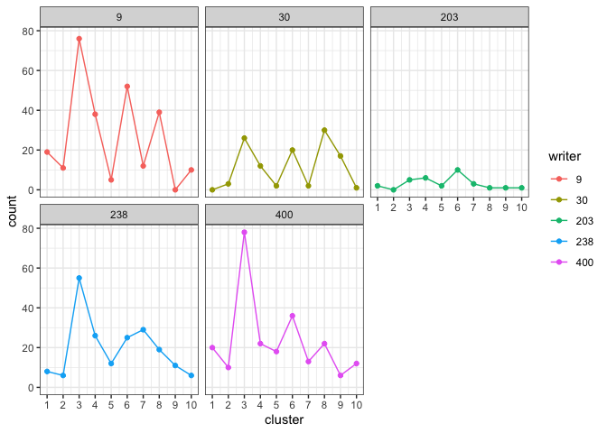
View the posterior probabilities of writership.
analysis$posterior_probabilities
#>         known_writer w0030_s03_pWOZ_r01
#> 1 known_writer_w0009                  0
#> 2 known_writer_w0030                  1
#> 3 known_writer_w0238 0In practice, we would not know who wrote a questioned document, but in research we often perform tests to evaluate models using data where we know the ground truth. Because in this example, we know the true writer of each questioned document, we can measure the accuracy of the model. We define accuracy as the average posterior probability assigned to the true writer. The accuracy of our model is
calculate_accuracy(analysis)
#> [1] 1