This Vignette will walk you through the usage of the Hypergate R package.
Installing dependencies:
install.packages(c("sp", "polyclip", "rgeos"))
source("https://bioconductor.org/biocLite.R")
biocLite("flowCore")
Installing the package from github:
This loads 2000 datapoints randomly sampled from the Samusik_01 dataset (available from FlowRepository accession number FR-FCM-ZZPH). This object is a list which includes as elements
fs_src a flowSet with 1 flowFrame corresponding to the data subset
xp_src a matrix corresponding to the expression of the data subset. Rownames correspond to event numbers in the unsampled dataset. Colnames correspond to protein targets (or other information e.g. events’ manually-annotated labels)
labels numeric vector encoding manually-annotated labels, with the value -1 for ungated events. The text labels for the gated populations are available from FlowRepostiry
regular_channels A subset of colnames(Samusik_01_subset$xp_src) that corresponds to protein targets
tsne A 2D-tSNE ran on the whole dataset and subsampled to 2000 events
Hypergate requires in particular as its arguments
an expression matrix (which we have as Samusik_01_subset$xp_src)
a vector specifying which events to attempt to gate on. This section discusses ways to achieve this point
We included in the package a function with a rudimentary (hopefully sufficient) interface that allows for the selection of a cell subset of interest from a 2D biplot by drawing a polygon around it using the mouse. Since this function is interactive we cannot execute it in this Vignette but an example call would be as such (feel free to try it):
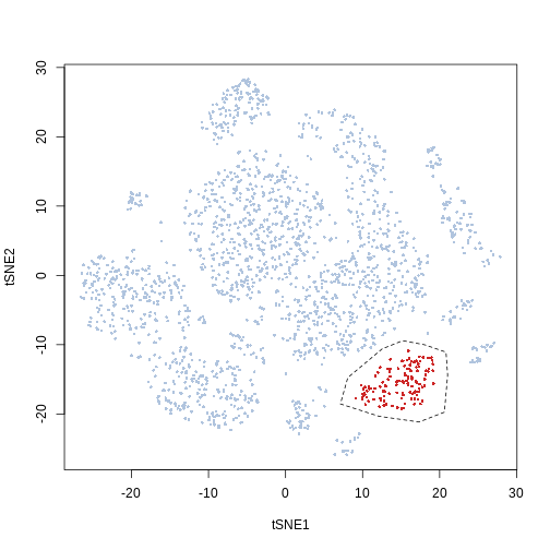
For this tutorial we define manually the polygon instead
x = c(12.54, 8.08, 7.12, 12.12, 17.32, 20.62, 21.04, 20.83, 18.07,
    15.2)
y = c(-10.61, -14.76, -18.55, -20.33, -21.16, -19.74, -14.4,
    -11.08, -10.02, -9.42)
pol = list(x = x, y = y)
library("sp")
gate_vector = sp::point.in.polygon(Samusik_01_subset$tsne[, 1],
    Samusik_01_subset$tsne[, 2], pol$x, pol$y)
plot(Samusik_01_subset$tsne, pch = 16, cex = 0.5, col = ifelse(gate_vector ==
    1, "firebrick3", "lightsteelblue"))
polygon(pol, lty = 2)Another option to define a cell cluster of interest is to use the output of a clustering algorithm. Popular options for cytometry include FlowSOM (available from Bioconductor) or Phenograph (available from the cytofkit package from Bioconductor). An example call for Rphenograph is below:
require(Rphenograph)
set.seed(5881215)
clustering = Rphenograph(Samusik_01_subset$xp_src[, Samusik_01_subset$regular_channels])
cluster_labels = membership(clustering[[2]])
In this Vignette we use the simpler kmeans option instead:
In this example we can see that the kmeans cluster 20 corresponds to the population we manually selected from the t-SNE biplot
plot(Samusik_01_subset$tsne, col = ifelse(cluster_labels == 20,
    "firebrick3", "lightsteelblue"), pch = 16, cex = 0.5)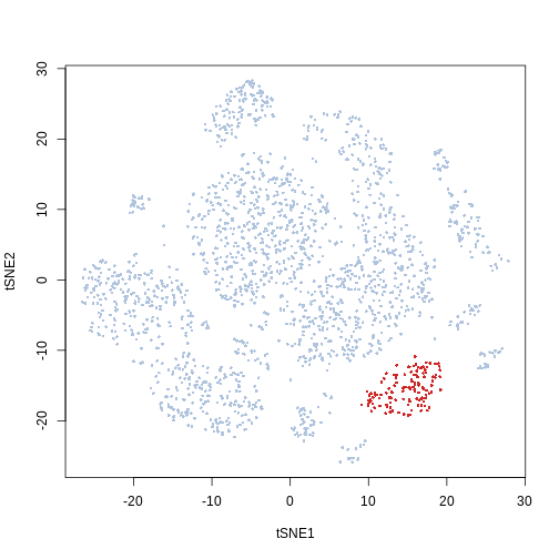
The function to optimize gating strategies is hypergate. Its main arguments are xp (a numeric matrix encoding expression), gate_vector (a vector with few unique values), level (specificies what value of gate_vector to gate upon, i.e. events satisfying gate_vector==level will be gated in)
hg_output = hypergate(xp = Samusik_01_subset$xp_src[, Samusik_01_subset$regular_channels],
gate_vector = gate_vector, level = 1, verbose = FALSE)The following function allows to subset an expression matrix given a return from Hypergate. The new matrix needs to have the same column names as the original matrix.
gating_predicted = subset_matrix_hg(hg_output, Samusik_01_subset$xp_src[,
Samusik_01_subset$regular_channels])table(ifelse(gating_predicted, "Gated-in", "Gated-out"), ifelse(gate_vector ==
1, "Events of interest", "Others"))| Events of interest | Others | |
|---|---|---|
| Gated-in | 116 | 0 |
| Gated-out | 10 | 1874 |
Another option, which offers more low-level control, is to examine for each datapoint whether they pass the threshold for each parameter. The function to obtain such a boolean matrix is boolmat. Here our gating strategy specifies SiglecF+cKit-Ly6C-. We would thus obtain a 3-columns x 2000 (the number of events) rows
bm = boolmat(gate = hg_output, xp = Samusik_01_subset$xp_src[,
    Samusik_01_subset$regular_channels])
head(bm)
## SiglecF_min cKit_max Ly6C_max
## 20 FALSE TRUE TRUE
## 28 FALSE TRUE TRUE
## 70 FALSE FALSE TRUE
## 110 TRUE FALSE FALSE
## 120 FALSE TRUE FALSE
## 159 FALSE TRUE FALSE| Events of interest | Others | |
|---|---|---|
| Gated-out because of SiglecF | 9 | 1829 |
| SiglecF above threshold | 117 | 45 |
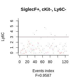
The following function will plot the output of Hypergate. Arguments are
gate an object returned by Hypergate
xp an expression matrix whose columns are named similarly as the ones used to create the gate object
gate_vector and level to specify which events are “of interest”
highlight a color that will be used to highlight the events of interest
plot_gating_strategy(gate = hg_output, xp = Samusik_01_subset$xp_src[,
    Samusik_01_subset$regular_channels], gate_vector = gate_vector,
    level = 1, highlight = "firebrick3")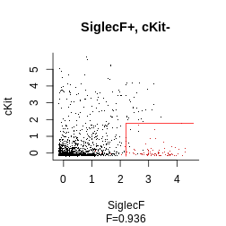
Another important point to consider is how the F\(\beta\)-score increases with each added channel. This gives an idea of how many channels are required to reach a close-to-optimal gating strategy.
This will identify at which steps the parameters were first activated and optimized:
f_values_vs_number_of_parameters = c(F_beta(rep(TRUE, nrow(Samusik_01_subset$xp_src)),
    gate_vector == 1), hg_output$f[c(apply(hg_output$pars.history[,
    hg_output$active_channels], 2, function(x) min(which(x !=
    x[1]))) - 1, nrow(hg_output$pars.history))][-1])
barplot(rev(f_values_vs_number_of_parameters), names.arg = rev(c("Initialization",
    paste("+ ", sep = "", hg_output$active_channels))), las = 3,
    mar = c(10, 4, 1, 1), horiz = TRUE, xlab = "Cumulative F1-score")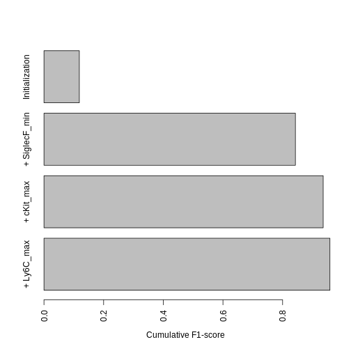
This graph tells us that the biggest increase is by far due to SiglecF+, while the lowest is due to Ly6C-.
The previous graph only shows how the F-value evolved during optimization, but what we really want to know is how much each parameter contributes to the final output (sometimes a parameter will have a big impact at the early steps of the optimization but will become relatively unimportant towards the end, if multiple other parameters collectively account for most of its discriminatory power). We use the following function to assess this, which measures how much performances lower when a parameter is ignored. The more the performances lower, the more important the parameter is.
contributions = channels_contributions(gate = hg_output, xp = Samusik_01_subset$xp_src[,
    Samusik_01_subset$regular_channels], gate_vector = gate_vector,
    level = 1, beta = 1)
barplot(contributions, las = 3, mar = c(10, 4, 1, 1), horiz = TRUE,
    xlab = "F1-score deterioration when the parameter is ignored")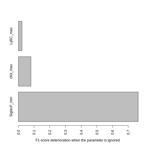
Since Ly6C contributes very little, we may want to ignore it to obtain a shorter gating strategy. We could keep the current threshold values for the other parameters, but it is best to re-compute the other thresholds to account for the loss of some parameters. To do that we use the following function:
hg_output_polished = reoptimize_strategy(gate = hg_output, channels_subset = c("SiglecF_min",
    "cKit_max"), xp = Samusik_01_subset$xp_src[, Samusik_01_subset$regular_channels],
    gate_vector = gate_vector, level = 1)
Finally, we get to plot our final strategy:
plot_gating_strategy(gate = hg_output_polished, xp = Samusik_01_subset$xp_src[,
    Samusik_01_subset$regular_channels], gate_vector = gate_vector,
    level = 1, highlight = "firebrick3")
Thanks to a nice contribution for SamGG on github, there are three functions that make the outputs more readable:
## [1] "SiglecF+, cKit-, Ly6C-"## [1] "SiglecF >= 2.21, cKit <= 1.77, Ly6C <= 2.98"## channels sign comp threshold
## SiglecF_min SiglecF + >= 2.208221
## cKit_max cKit - <= 1.770901
## Ly6C_max Ly6C - <= 2.983523# Fscores can be retrieved when the same parameters given to
# hypergate() are given to hgate_info():
hg_out_info = hgate_info(hg_output, xp = Samusik_01_subset$xp_src[,
Samusik_01_subset$regular_channels], gate_vector = gate_vector,
level = 1)
hg_out_info## channels sign comp threshold deltaF Fscore1D Fscore
## SiglecF_min SiglecF + >= 2.208221 0.76351765 0.8125 0.8125
## cKit_max cKit - <= 1.770901 0.07988981 0.1294 0.9360
## Ly6C_max Ly6C - <= 2.983523 0.02267769 0.1809 0.9587## [1] "0.8125, 0.936, 0.9587"Some comments about potential questions on your own projects (raised by QBarbier):
Anything that would be relevant for a gating strategy should be used as an input. So usually any phenotypic channel would be included. If you know that you would not use certain parameters on subsequent experiments (for instance if the staining is intracellular and you plan to sort a live population and thus cannot permeabilize your cells), you should exclude the corresponding channels. I usually do not use channels that were used in pre-gating steps (e.g. CD45 for immune cells). Finally, if you plan to use flow cytometry and use hypergate on a CyTOF dataset, you probably want to discard the Cell_length channel.
It depends on how much RAM your computer has. If that is an issue I suggest downsampling to (e.g.) 1000 positive cells and a corresponding number of negative cells. The hgate_sample function can help you achieve this:
set.seed(123)  ## Makes the subsampling reproducible
gate_vector = Samusik_01_subset$labels
subsample = hgate_sample(gate_vector = gate_vector, level = 5,
    size = 100)  ## Subsample 100 events from population #5 (Classical monocytes), and a corresponding number of negative events
tab = table(ifelse(subsample, "In", "Out"), ifelse(Samusik_01_subset$labels ==
    5, "Positive pop.", "Negative pop."))
tab[1, ]/colSums(tab)  ## Fraction of subsampled events for positive and negative populations
## Negative pop. Positive pop.
## 0.3204976 0.3205128xp = Samusik_01_subset$xp_src[, Samusik_01_subset$regular_channels]
hg = hypergate(xp = xp[subsample, ], gate_vector = gate_vector[subsample],
level = 5) ## Runs hypergate on a subsample of the input matrix
gating_heldout = subset_matrix_hg(hg, xp[!subsample, ]) ## Applies the gate to the held-out data
table(ifelse(gating_heldout, "Gated in", "Gated out"), ifelse(Samusik_01_subset$labels[!subsample] ==
5, "Positive pop.", "Negative pop."))##
## Negative pop. Positive pop.
## Gated in 37 192
## Gated out 1110 20