In the generalized Roy model, the marginal treatment effect (MTE) can
be used as a building block for constructing conventional causal
parameters such as the average treatment effect (ATE) and the average
treatment effect on the treated (ATT). Given a treatment selection
equation and an outcome equation, the function mte()
estimates the MTE via the semiparametric local instrumental variables
(localIV) method or the normal selection model. The function
mte_at() evaluates MTE at different values of the latent
resistance u with a given X = x, and the
function mte_tilde_at() evaluates MTE projected onto the
estimated propensity score. The function ace() estimates
population-level average causal effects such as ATE, ATT, or the
marginal policy relevant treatment effect (MPRTE).
Main References
Heckman, James J., Sergio Urzua, and Edward Vytlacil. 2006. “Understanding Instrumental Variables in Models with Essential Heterogeneity.” The Review of Economics and Statistics 88(3):389-432.
Zhou, Xiang and Yu Xie. 2019. “Marginal Treatment Effects from A Propensity Score Perspective.” Journal of Political Economy, 127(6): 3070-3084.
Zhou, Xiang and Yu Xie. 2020. “Heterogeneous Treatment Effects in the Presence of Self-selection: a Propensity Score Perspective.” Sociological Methodology.
You can install the released version of localIV from CRAN with:
install.packages("localIV")And the development version from GitHub with:
# install.packages("devtools")
devtools::install_github("xiangzhou09/localIV")Below is a toy example illustrating the use of mte() to
fit an MTE model using the local IV method.
library(localIV)
mod <- mte(selection = d ~ x + z, outcome = y ~ x, data = toydata, bw = 0.2)
# fitted propensity score model
summary(mod$ps_model)
#>
#> Call:
#> glm(formula = selection, family = binomial("probit"), data = mf_s)
#>
#> Deviance Residuals:
#> Min 1Q Median 3Q Max
#> -3.4345 -0.6555 0.0115 0.6392 3.3983
#>
#> Coefficients:
#> Estimate Std. Error z value Pr(>|z|)
#> (Intercept) 0.01798 0.01580 1.138 0.255
#> x 0.95263 0.02065 46.124 <2e-16 ***
#> z 1.00431 0.02088 48.094 <2e-16 ***
#> ---
#> Signif. codes: 0 '***' 0.001 '**' 0.01 '*' 0.05 '.' 0.1 ' ' 1
#>
#> (Dispersion parameter for binomial family taken to be 1)
#>
#> Null deviance: 13862.7 on 9999 degrees of freedom
#> Residual deviance: 8217.1 on 9997 degrees of freedom
#> AIC: 8223.1
#>
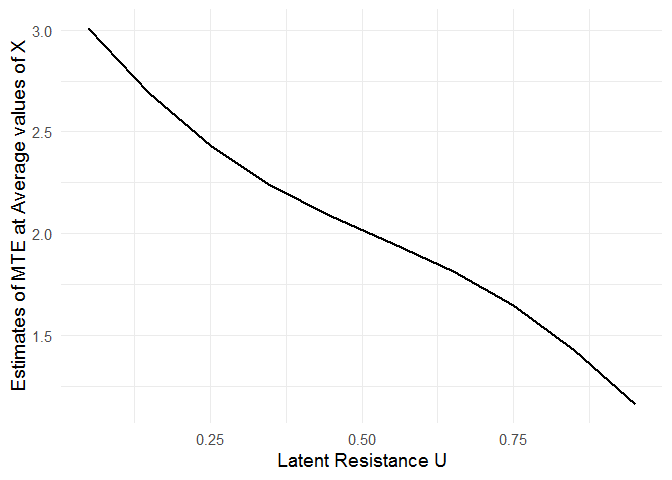
#> Number of Fisher Scoring iterations: 5After fitting the MTE model, the mte_at() function can
be used to examine treatment effect heterogeneity as a function of the
latent resistance u.
mte_vals <- mte_at(u = seq(0.05, 0.95, 0.1), model = mod)

# install.packages("ggplot2")
library(ggplot2)

ggplot(mte_vals, aes(x = u, y = value)) +
  geom_line(size = 1) +
  xlab("Latent Resistance U") +
  ylab("Estimates of MTE at Average values of X") +
  theme_minimal(base_size = 14)
The mte_tilde_at() function estimates the “MTE tilde”,
i.e., the expected treatment effect conditional on the propensity score
p and the latent resistance u. It reveals treatment
effect heterogeneity as a function of both p and
u.
u <- p <- seq(0.05, 0.95, 0.1)
mte_tilde <- mte_tilde_at(p, u, model = mod)

# heatmap showing MTE_tilde(p, u)
ggplot(mte_tilde$df, aes(x = u, y = p, fill = value)) +
  geom_tile() +
  scale_fill_gradient(name = expression(widetilde(MTE)(p, u)), low = "yellow", high = "blue") +
  xlab("Latent Resistance U") +
  ylab("Propensity Score p(Z)") +
  theme_minimal(base_size = 14)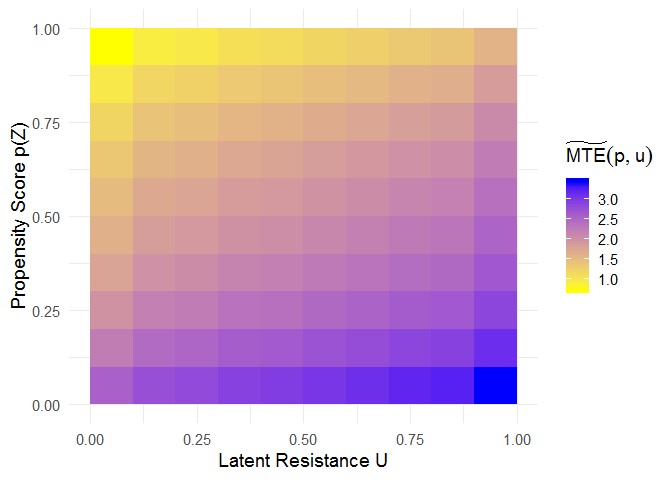
When u = p, the “MTE tilde” corresponds to the marginal policy relevant treatment effect (MPRTE) as a function of p.
mprte_tilde_df <- subset(mte_tilde$df, p == u)

# heatmap showing MPRTE_tilde(p)
ggplot(mprte_tilde_df, aes(x = u, y = p, fill = value)) +
  geom_tile() +
  scale_fill_gradient(name = expression(widetilde(MPRTE)(p)), low = "yellow", high = "blue") +
  xlab("Latent Resistance U") +
  ylab("Propensity Score p(Z)") +
  theme_minimal(base_size = 14)
# decomposition of MPRTE_tilde(p) into the p-component and the u-component

# install.packages(c("dplyr", "tidyr"))
library(dplyr)
library(tidyr)

mprte_tilde_df %>%
  pivot_longer(cols = c(u_comp, p_comp, value)) %>%
  mutate(name = recode_factor(name,
         `value` = "MPRTE(p)",
         `p_comp` = "p(Z) component",
         `u_comp` = "U component")) %>%
  ggplot(aes(x = p, y = value)) +
  geom_line(aes(linetype = name), size = 1) +
  scale_linetype("") +
  xlab("Propensity Score p(Z)") +
  ylab("Treatment Effect") +
  theme_minimal(base_size = 14)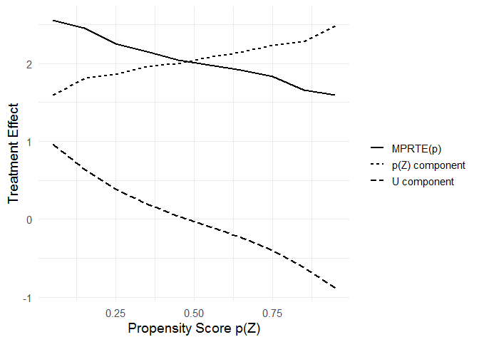
Finally, the ace() function can be used to estimate
population-level Average Causal Effects including ATE, ATT, ATU, and the
marginal policy relevant treatment effect (MPRTE). When estimating the
MPRTE at the population level, policy needs to be specified
as an expression representing a univariate function of
p.
ate <- ace(mod, "ate")
att <- ace(mod, "att")
atu <- ace(mod, "atu")
mprte1 <- ace(mod, "mprte")
mprte2 <- ace(mod, "mprte", policy = p)
mprte3 <- ace(mod, "mprte", policy = 1-p)
mprte4 <- ace(mod, "mprte", policy = I(p<0.25))

c(ate, att, atu, mprte1, mprte2, mprte3, mprte4)
#>                ate                att                atu           mprte: 1
#>           2.045050           2.525198           1.559401           2.048361
#>           mprte: p       mprte: 1 - p mprte: I(p < 0.25)
#>           1.826024           2.272419           2.486643