- When comparing nested models
- Associations between variables within clusters
- Associations between variables between clusters
- Caterpillar plots
Multilevel and mixed effects models often require specialized data
pre-processing and further post-estimation derivations and graphics to
gain insight into model results. mlmtools is a suite of
pre- and post-estimation tools for multilevel models in R. The package’s
post-estimation tools are designed to work with models estimated using
lme4’s lmer function, which fits linear mixed effects
regression models. Although nearly all the functions provided in the
mlmtools package exist as singleton functions within other
R packages, they are often improved in mlmtools and more
accessible by being located within a multilevel modeling specific
package.
The package was developed by Laura Jamison, Jessican Mazen, Erik Ruzek, and Gus Sjobek.
To install the latest release version (1.0.0) from GitHub with:
# install.packages("devtools")
devtools::install_github("lj5yn/mlmtools")Working with the included data, we briefly show how some of the included functions can be used.
# data
library(mlmtools)
library(lme4)
#> Loading required package: Matrix
data("instruction")

# fit variance components model
fit1 <- lmer(mathgain ~ 1 + (1|classid), instruction)

# intraclass correlation coefficient
ICCm(fit1)
#> Likeness of mathgain values of units in the same classid factor: 0.149

# group-mean center mathkind
center(instruction, x="mathkind", grouping = "classid")
#> The following variables (deviation, group summary) were added to the dataset:
#>  classid_mathkind.devcmn classid_mathkind.cmn
#> See mlmtools documentation for detailed description of variables added.

# add group-mean centered and group mean as predictors
fit2 <- lmer(mathgain ~ classid_mathkind.devcmn + classid_mathkind.cmn + (1|classid), instruction)

# variance explained by adding predictor
varCompare(fit2, fit1)
#> fit2 explains 31.08% more variance than fit1

# test model assumptions
mlm_assumptions(fit2)
#> Homogeneity of variance assumption met.
#>
#> Model contains fewer than 2 terms, multicollinearity cannot be assessed.
#>
#> No outliers detected.
#>
#> Visually inspect all 4 plot types by calling them from the object created by mlm_assumptions() such as object$fitted.residual.plot and object$resid.normality.plot. linearity.plots and resid.component.plots may contain more than one plot depending on the model specified. Check how many there are, for example using length(object$linearity.plots). Then inspect each plot within each object, for example using object$linearity.plots[[1]] to access the first plot within the linearity.plots list.
#>
#> See ?mlm_assumptions for more details and resources.
#>
#> $linearity.plots
#> $linearity.plots[[1]]
#>
#> $linearity.plots[[2]]
#>
#>
#> $homo.test
#> Analysis of Variance Table
#>
#> Response: model.Res2
#>             Df     Sum Sq Mean Sq F value  Pr(>F)
#> classid      1    6872688 6872688  3.4323 0.06418 .
#> Residuals 1188 2378796930 2002354
#> ---
#> Signif. codes:  0 '***' 0.001 '**' 0.01 '*' 0.05 '.' 0.1 ' ' 1
#>
#> $fitted.residual.plot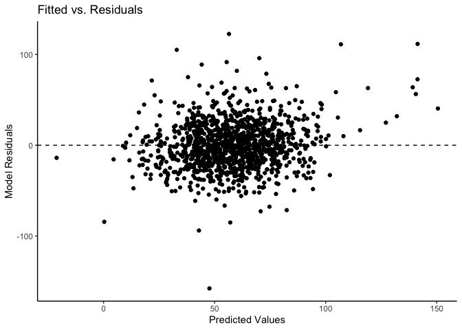
#>
#> $outliers
#> [1] "664"
#>
#> $resid.normality.plot
#>
#> $resid.component.plots
#> $resid.component.plots[[1]]
#> `geom_smooth()` using method = 'gam' and formula 'y ~ s(x, bs = "cs")'
#>
#> $resid.component.plots[[2]]
#> `geom_smooth()` using method = 'gam' and formula 'y ~ s(x, bs = "cs")'
#>
#>
#> $multicollinearity
#> [1] "Model contains fewer than 2 terms, multicollinearity cannot be assessed.\n"
#>
#> attr(,"class")
#> [1] "mlm_assumptions"

# variance explained by the model
rsqmlm(fit2)
#> 24.58% of the total variance is explained by the fixed effects.
#> 37.73% of the total variance is explained by both fixed and random effects.Rich visualizations of associations can be had along with caterpillar plots, which graph the 95% prediction intervals for the random effects.
# visualize between-group association
betweenPlot(x = "mathkind", y = "mathgain", grouping = "classid", dataset = instruction, xlab = "Kindergarten Math Score", ylab = "Gain in Math Score")
# visualze within-group association
withinPlot(x = "mathkind", y = "mathgain", grouping = "classid", dataset = instruction)
# caterpillar plot
caterpillarPlot(fit2, grouping = "classid")
#> [1] "classid"