![]()
![]()
This package implements the d3-force algorithm developed by Mike Bostock in R, thus providing a way to run many types of particle simulations using its versatile interface.
While the first goal is to provide feature parity with its JavaScript
origin, the intentions is to add more forces, constraints, etc. down the
line. While d3-force is most well-known as a layout engine for
visualising networks, it is capable of much more. Therefore,
particles is provided as a very open framework to play
with. Eventually ggraph will
provide some shortcut layouts based on particles with the
aim of facilitating network visualisation.
particles builds upon the framework provided by tidygraph
and adds a set of verbs that defines the simulation:
simulate() : Creates a simulation based on the input
graph, global parameters, and a genesis function that sets up the
initial conditions of the simulation.wield() : Adds a force to the simulation. All forces
implemented in d3-force are available as well as some additionals.impose() : Adds a constraint to the simulation. This
function is a departure from d3-force, as d3-force only allowed for
simple fixing of x and/or y coordinates through the use of the fx and fy
accessors. particles formalises the use of simulation
constraints and adds new functionalities.evolve() : Progresses the simulation, either a
predefined number of steps, or until the simulated annealing has cooled
down.A recreation of the Les Miserable network in https://bl.ocks.org/mbostock/4062045
library(tidyverse)
library(ggraph)
library(tidygraph)
library(particles)
# Data preparation
d3_col <- c(
'0' = "#98df8a",
'1' = "#1f77b4",
'2' = "#aec7e8",
'3' = "#ff7f0e",
'4' = "#ffbb78",
'5' = "#2ca02c",
'6' = "#d62728",
'7' = "#ff9896",
'8' = "#9467bd",
'9' = "#c5b0d5",
'10' = "#8c564b"
)
raw_data <- 'https://gist.githubusercontent.com/mbostock/4062045/raw/5916d145c8c048a6e3086915a6be464467391c62/miserables.json'
miserable_data <- jsonlite::read_json(raw_data, simplifyVector = TRUE)
miserable_data$nodes$group <- as.factor(miserable_data$nodes$group)
miserable_data$links <- miserable_data$links |>
mutate(from = match(source, miserable_data$nodes$id),
to = match(target, miserable_data$nodes$id))
# Actual particles part
mis_graph <- miserable_data |>
simulate() |>
wield(link_force) |>
wield(manybody_force) |>
wield(center_force) |>
evolve() |>
as_tbl_graph()
# Plotting with ggraph
ggraph(mis_graph, 'nicely') +
geom_edge_link(aes(width = sqrt(value)), colour = '#999999', alpha = 0.6) +
geom_node_point(aes(fill = group), shape = 21, colour = 'white', size = 4,
stroke = 1.5) +
scale_fill_manual('Group', values = d3_col) +
scale_edge_width('Value', range = c(0.5, 3)) +
coord_fixed() +
theme_graph()
#> Warning: Existing variables `x`, `y` overwritten by layout variables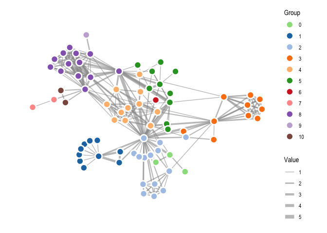
If you intend to follow the steps of the simulation it is possible to attach an event handler that gets called ofter each generation of the simulation. If the handler produces a plot the result will be an animation of the simulation:
# Random overlapping circles
graph <- as_tbl_graph(igraph::erdos.renyi.game(100, 0)) |>
  mutate(x = runif(100) - 0.5,
         y = runif(100) - 0.5,
         radius = runif(100, min = 0.1, 0.2))

# Plotting function
graph_plot <- function(sim) {
  gr <- as_tbl_graph(sim)
  p <- ggraph(gr, layout = as_tibble(gr)) +
    geom_node_circle(aes(r = radius), fill = 'forestgreen', alpha = 0.5) +
    coord_fixed(xlim = c(-2.5, 2.5), ylim = c(-2.5, 2.5)) +
    theme_graph()
  plot(p)
}

# Simulation
graph %>% simulate(velocity_decay = 0.7, setup = predefined_genesis(x, y)) |>
  wield(collision_force, radius = radius, n_iter = 2) |>
  wield(x_force, x = 0, strength = 0.002) |>
  wield(y_force, y = 0, strength = 0.002) |>
  evolve(on_generation = graph_plot)
Click here for resulting animation (GitHub don’t allow big gifs in readme)
You can install particles from CRAN using
install.packages("particles") or alternatively install the
development version from github with:
# install.packages("devtools")
devtools::install_github("thomasp85/particles")particles wouldn’t exist and without d3 in general the
world would be a sadder place.manbody_force and collision_force is a
modification of the implementation made by
Andrei Kashcha and made available under MIT license. Big thanks to
Andrei as well.