![]()
This package provides functions to evaluate moments of ratios (and products) of quadratic forms in normal variables, specifically using recursive algorithms developed by Bao and Kan (2013) and Hillier et al. (2014). Generating functions for these moments are closely related to the top-order zonal and invariant polynomials of matrix arguments. It also provides some functions to evaluate distribution and density functions of simple ratios of quadratic forms in normal variables using several methods from Imhof (1961), Hillier (2001), Forchini (2002, 2005), Butler and Paolella (2008), and Broda and Paolella (2009).
There exist a couple of Matlab programs developed by Raymond Kan (available from https://www-2.rotman.utoronto.ca/~kan/) for evaluating the moments, but this R package is an independent project (not a fork or translation) and has different functionalities, including evaluation of moments of multiple ratios of a particular form and scaling to avoid numerical overflow. This has originally been developed for a biological application, specifically for evaluating average evolvability measures in evolutionary quantitative genetics (Watanabe, 2023), but can be used for a broader class of statistics.
WARNING Installation size of this package can be very large (>100 MB on Linux and macOS; ~3 MB on Windows with a recent version (>= 4.2) of Rtools), as it involves lots of RcppEigen functions.
## Install devtools first:
# install.packages("devtools")

## Recommended installation (pandoc required):
devtools::install_github("watanabe-j/qfratio", dependencies = TRUE, build_vignettes = TRUE)

## Minimal installation:
# devtools::install_github("watanabe-j/qfratio")Imports: Rcpp, MASS, stats
LinkingTo: Rcpp, RcppEigen
Suggests: mvtnorm, CompQuadForm, graphics, testthat (>= 3.0.0),
knitr, rmarkdownIf installing from source, you also need pandoc for correctly building the vignette. For pandoc < 2.11, pandoc-citeproc is required as well. (Never mind if you use RStudio, which appears to have them bundled.)
This package has two major functionalities: evaluating moments and distribution function of ratios of quadratic forms in normal variables.
This functionality concerns evaluation of the following moments: \(\mathrm{E} \left( \left( \mathbf{x}^T \mathbf{A} \mathbf{x} \right)^p / \left( \mathbf{x}^T \mathbf{B} \mathbf{x} \right)^q \right)\) and \(\mathrm{E} \left( \left( \mathbf{x}^T \mathbf{A} \mathbf{x} \right)^p / \left( \mathbf{x}^T \mathbf{B} \mathbf{x} \right)^q \left( \mathbf{x}^T \mathbf{D} \mathbf{x} \right)^r \right)\), where \(\mathbf{x} \sim N_n \left(\boldsymbol{\mu}, \boldsymbol{\Sigma}\right)\).
These quantities are evaluated by qfrm(A, B, p, q, ...) and qfmrm(A, B, D, p, q, r, ...). Because they are evaluated as partial sums of infinite series (Smith, 1989, 1993; Hillier et al., 2009, 2014; Bao and Kan, 2013), the evaluation results come with an error bound (where available), and a plot method is defined for inspecting numerical convergence.
## Simple matrices
nv <- 4
A <- diag(1:nv)
B <- diag(sqrt(nv:1))

## Expectation of (x^T A x)^2 / (x^T x)^2 where x ~ N(0, I)
qfrm(A, p = 2)
#>
#>  Moment of ratio of quadratic forms
#>
#> Moment = 6.666667
#> This value is exact

## Compare with Monte Carlo mean
mean(rqfr(1000, A = A, p = 2))
#> [1] 6.641507

## Expectation of (x^T A x)^1/2 / (x^T x)^1/2
(mom_A0.5 <- qfrm(A, p = 1/2))
#>
#>  Moment of ratio of quadratic forms
#>
#> Moment = 1.567224, Error = -6.335806e-19 (one-sided)
#> Possible range:
#>  1.56722381 1.56722381

## Monte Carlo mean
mean(rqfr(1000, A = A, p = 1/2))
#> [1] 1.569643

plot(mom_A0.5)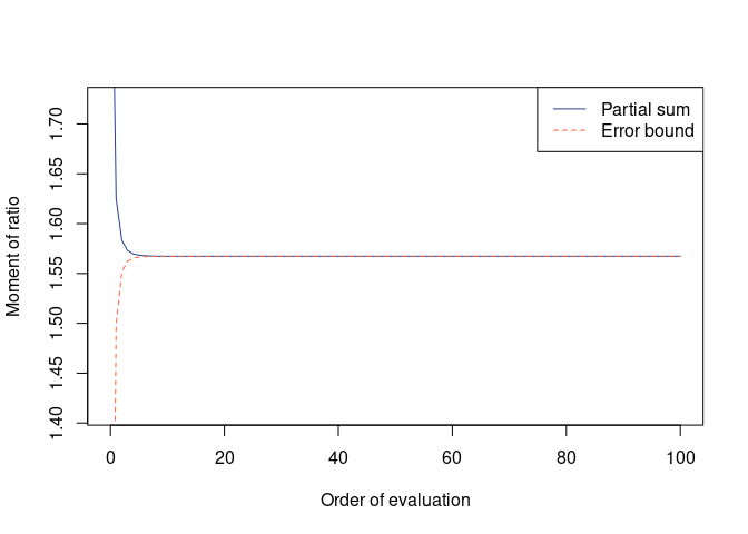
## Expectation of (x^T x) / (x^T A^-1 x)
##   = "average conditional evolvability"
(avr_cevoA <- qfrm(diag(nv), solve(A)))
#>
#>  Moment of ratio of quadratic forms
#>
#> Moment = 2.11678, Error = 2.768619e-15 (one-sided)
#> Possible range:
#>  2.11677962 2.11677962

mean(rqfr(1000, A = diag(nv), B = solve(A), p = 1))
#> [1] 2.071851
plot(avr_cevoA)
## Expectation of (x^T x)^2 / (x^T A x) (x^T A^-1 x)
##   = "average autonomy"
(avr_autoA <- qfmrm(diag(nv), A, solve(A), p = 2, q = 1, r = 1))
#>
#>  Moment of ratio of quadratic forms
#>
#> Moment = 0.8416553
#> Error bound unavailable; recommended to inspect plot() of this object

mean(rqfmr(1000, A = diag(nv), B = A, D = solve(A), p = 2, q = 1, r = 1))
#> [1] 0.8377911
plot(avr_autoA)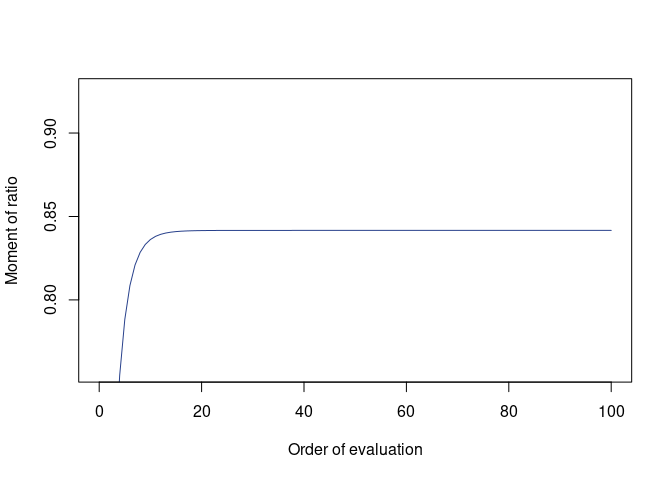
## Expectation of (x^T A B x) / ((x^T A^2 x) (x^T B^2 x))^1/2
##   = "average response correlation"
## whose Monte Carlo evaluation is called the "random skewers" analysis,
## while this is essentially an analytic solution (with slight truncation error)
(avr_rcorA <- qfmrm(crossprod(A, B), crossprod(A), crossprod(B),
                    p = 1, q = 1/2, r = 1/2))
#>
#>  Moment of ratio of quadratic forms
#>
#> Moment = 0.8462192
#> Error bound unavailable; recommended to inspect plot() of this object

mean(rqfmr(1000, A = crossprod(A, B), B = crossprod(A), D = crossprod(B),
           p = 1, q = 1/2, r = 1/2))
#> [1] 0.8467811
plot(avr_rcorA)
## More complex (but arbitrary) example
## Expectation of (x^T A x)^2 / (x^T B x)^3 where x ~ N(mu, Sigma)
mu <- 1:nv / nv
Sigma <- diag(runif(nv) * 3)
(mom_A2B3 <- qfrm(A, B, p = 2, q = 3, mu = mu, Sigma = Sigma,
                  m = 500, use_cpp = TRUE))
#>
#>  Moment of ratio of quadratic forms
#>
#> Moment = 0.510947, Error = 0 (two-sided)
#> Possible range:
#>  0.510946975 0.510946975
plot(mom_A2B3)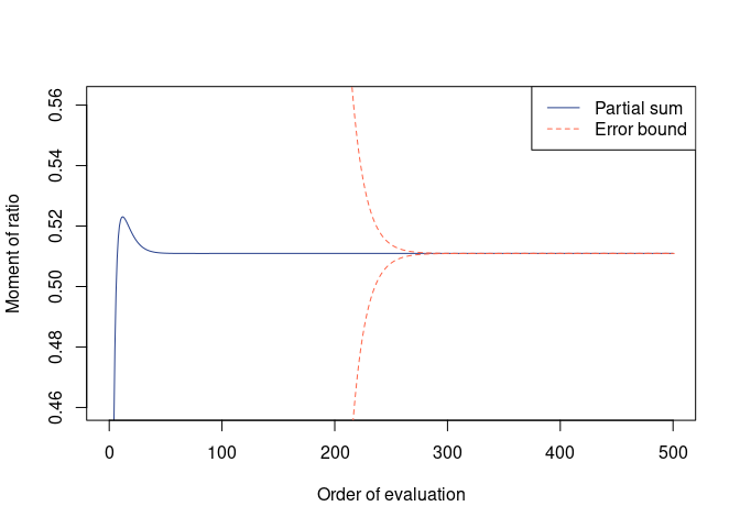
This functionality concerns evaluation of the (cumulative) distribution function, probability density, and quantiles of \(\left( \mathbf{x}^T \mathbf{A} \mathbf{x} / \mathbf{x}^T \mathbf{B} \mathbf{x} \right) ^ p\), where \(\mathbf{x} \sim N_n \left(\boldsymbol{\mu}, \boldsymbol{\Sigma}\right)\).
These are implemented in pqfr(quantile, A, B, p, ...), dqfr(quantile, A, B, p, ...), and qqfr(probability, A, B, p, ...), whose usage mimics that of regular distribution-related functions.
## Example parameters
nv <- 4
A <- diag(1:nv)
B <- diag(sqrt(nv:1))
mu <- 1:nv * 0.2
quantiles <- 0:nv + 0.5

## Distribution function and density of
## (x^T A x) / (x^T B x) where x ~ N(0, I)
pqfr(quantiles, A, B)
#> [1] 0.0000000 0.4349385 0.8570354 0.9816503 1.0000000
dqfr(quantiles, A, B)
#> [1] 0.00000000 0.57079928 0.21551262 0.06123152 0.00000000

## 95, 99, and 99.9 percentiles of the same
qqfr(c(0.05, 0.01, 0.001), A, B, lower.tail = FALSE)
#> [1] 3.111025 3.654857 3.921405

## Comparing profiles
qseq <- seq.int(1 / sqrt(nv) - 0.2, nv + 0.2, length.out = 100)

## Generate p-value sequences for
## (x^T A x) / (x^T B x) where x ~ N(0, I) vs
## (x^T A x) / (x^T B x) where x ~ N(mu, I)
pseq_central <- pqfr(qseq, A, B)
pseq_noncent <- pqfr(qseq, A, B, mu = mu)

## Graphical comparison
plot(qseq, type = "n", xlim = c(1 / sqrt(nv), nv), ylim = c(0, 1),
     xlab = "q", ylab = "F(q)")
lines(qseq, pseq_central, col = "royalblue4", lty = 1)
lines(qseq, pseq_noncent, col = "tomato", lty = 2)
legend("topleft", legend = c("central", "noncentral"),
       col = c("royalblue4", "tomato"), lty = 1:2)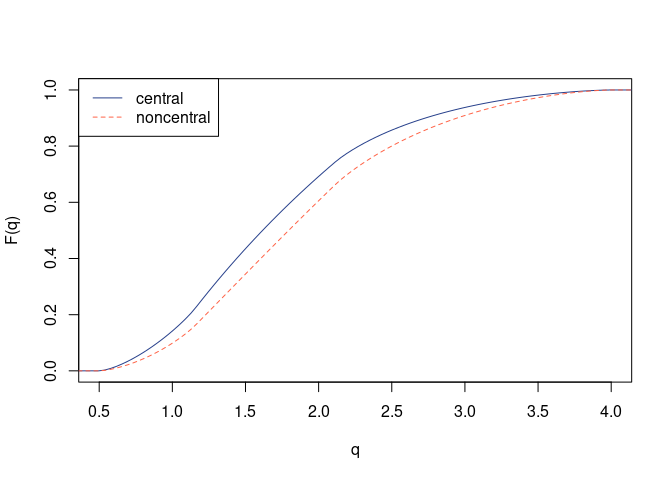
## Generate density sequences for
## (x^T A x) / (x^T B x) where x ~ N(0, I) vs
## (x^T A x) / (x^T B x) where x ~ N(mu, I)
dseq_central <- dqfr(qseq, A, B)
dseq_noncent <- dqfr(qseq, A, B, mu = mu)

## Graphical comparison
plot(qseq, type = "n", xlim = c(1 / sqrt(nv), nv), ylim = c(0, 0.7),
     xlab = "q", ylab = "f(q)")
lines(qseq, dseq_central, col = "royalblue4", lty = 1)
lines(qseq, dseq_noncent, col = "tomato", lty = 2)
legend("topright", legend = c("central", "noncentral"),
       col = c("royalblue4", "tomato"), lty = 1:2)
This package bundles selected C codes and part of config.ac from the GNU Scientific Library, whose copyright belongs to the original authors. See DESCRIPTION and individual code files in src/gsl for details. The redistribution complies with the GNU General Public License version 3.
Bao, Y. and Kan, R. (2013) On the moments of ratios of quadratic forms in normal random variables. Journal of Multivariate Analysis, 117, 229–245. doi:10.1016/j.jmva.2013.03.002.
Broda, S. and Paolella, M. S. (2009) Evaluating the density of ratios of noncentral quadratic forms in normal variables. Computational Statistics and Data Analysis, 53, 1264–1270. doi:10.1016/j.csda.2008.10.035.
Butler, R. W. and Paolella, M. S. (2008) Uniform saddlepoint approximations for ratios of quadratic forms. Bernoulli, 14, 140–154. doi:10.3150/07-BEJ6169.
Forchini, G. (2002) The exact cumulative distribution function of a ratio of quadratic forms in normal variables, with application to the AR(1) model. Econometric Theory, 18, 823–852. doi:10.1017/s0266466602184015.
Forchini, G. (2005) The distribution of a ratio of quadratic forms in noncentral normal variables. Communications in Statistics—Theory and Methods, 34, 999–1008. doi:10.1081/STA-200056855.
Hillier, G. (2001) The density of a quadratic form in a vector uniformly distributed on the n-sphere. Econometric Theory, 17, 1–28. doi:10.1017/S026646660117101X.
Hillier, G., Kan, R. and Wang, X. (2009) Computationally efficient recursions for top-order invariant polynomials with applications. Econometric Theory, 25, 211–242. doi:10.1017/S0266466608090075.
Hillier, G., Kan, R. and Wang, X. (2014) Generating functions and short recursions, with applications to the moments of quadratic forms in noncentral normal vectors. Econometric Theory, 30, 436–473. doi:10.1017/S0266466613000364.
Imhof, J. P. (1961) Computing the distribution of quadratic forms in normal variables. Biometrika, 48, 419–426. doi:10.2307/2332763.
Smith, M. D. (1989) On the expectation of a ratio of quadratic forms in normal variables. Journal of Multivariate Analysis, 31, 244–257. doi:10.1016/0047-259X(89)90065-1.
Smith, M. D. (1993) Expectations of ratios of quadratic forms in normal variables: Evaluating some top-order invariant polynomials. Australian Journal of Statistics, 35, 271–282. doi:10.1111/j.1467-842X.1993.tb01335.x.
Watanabe, J. (2023) Exact expressions and numerical evaluation of average evolvability measures for characterizing and comparing G matrices. Journal of Mathematical Biology, 86, 95. doi:10.1007/s00285-023-01930-8.