A quadmesh is a dense mesh describing a topologically continuous surface of 4-corner primitives. This is also known as a cell-based raster but in those contexts the corner coordinates and the continuous nature of the mesh is completely implicit. By making the dense mesh explicit we have access to every corner coordinate (not just the centres) which allows for some extra facilities over raster grids.
This package provides helpers for working with this mesh interpretation of gridded data to enable
mesh_plot).quadmesh()).triangmesh()).dquadmesh()).dtriangmesh()).shade3d()).bary_index()).triangulate_quads()).You can install:
install.packages("quadmesh")## install.packages("remotes")
remotes::install_github("hypertidy/quadmesh")Quadmesh provides a number of key features that are not readily available to more commonly used geospatial applications.
In raster there is an implicit “area-based” interpretion of the
extent and value of every cell. Coordinates are implicit, and
centre-based but the extent reflects a finite and constant
width and height.
library(quadmesh)
library(raster)
#> Loading required package: sp
r <- raster(matrix(1:12, 3), xmn = 0, xmx = 4, ymn = 0, ymx = 3)
qm <- quadmesh(r)

op <- par(xpd = NA)
plot(extent(r) + 0.5, type = "n", axes = FALSE, xlab = "", ylab = "")
plot(r, col = rep(c("palevioletred3", "aliceblue"), 6), add = TRUE)
text(coordinates(r), lab = seq_len(ncell(r)))
plot(extent(r), add = TRUE)

## with quadmesh there are 20 corner coordinates
points(t(qm$vb[1:2, ]), pch = "x", cex = 2)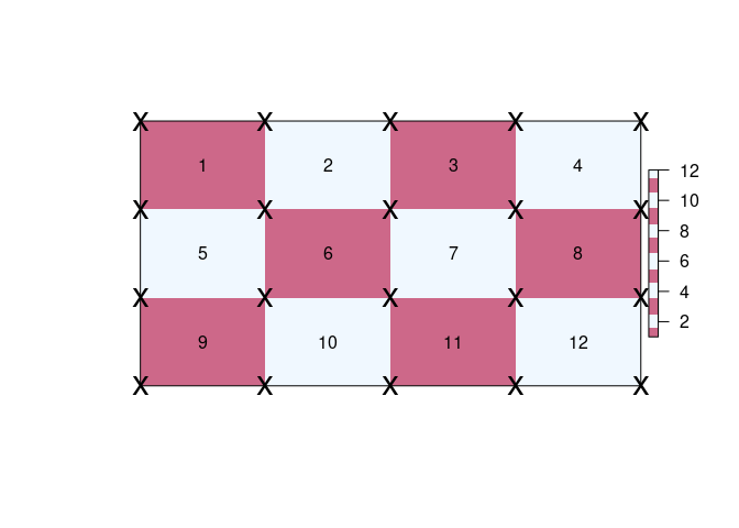
par(op)Every individual quad is described implicitly by index into the
unique corner coordinates. This format is built upon the
mesh3d class of the rgl package.
## coordinates, transpose here
qm$vb[1:2, ]
#>   [,1] [,2] [,3] [,4] [,5] [,6] [,7] [,8] [,9] [,10] [,11] [,12] [,13] [,14]
#> x    0    1    2    3    4    0    1    2    3     4     0     1     2     3
#> y    3    3    3    3    3    2    2    2    2     2     1     1     1     1
#>   [,15] [,16] [,17] [,18] [,19] [,20]
#> x     4     0     1     2     3     4
#> y     1     0     0     0     0     0

## indexes, also transpose
qm$ib
#>      [,1] [,2] [,3] [,4] [,5] [,6] [,7] [,8] [,9] [,10] [,11] [,12]
#> [1,]    1    2    3    4    6    7    8    9   11    12    13    14
#> [2,]    2    3    4    5    7    8    9   10   12    13    14    15
#> [3,]    7    8    9   10   12   13   14   15   17    18    19    20
#> [4,]    6    7    8    9   11   12   13   14   16    17    18    19
This separation of geometry (the 20 unique corner coordinates) and topology (12 sets of 4-index) is the key concept of a mesh and is found in many domains that involve computer graphics and modelling.
A quadmesh is centre-based, and each raster pixel occupies a little rectangle, but the centre-based interpretation is better described by a mesh of triangles.
Every centre point of the grid data is a node in this mesh, while the inside corners with their ambiguous value from 4 neighbouring cells are not explicit. Note that a triangulation can be top-left/bottom-right aligned as here, or bottom-left/top-right aligned, or be a mixture.
op <- par(xpd = NA)
plot(extent(r) + 0.5, type = "n", axes = FALSE, xlab = "", ylab = "")
plot(r, col = rep(c("palevioletred3", "aliceblue"), 6), add = TRUE)

tri <- triangmesh(r)
points(t(tri$vb[1:2, ]))
polygon(t(tri$vb[1:2, head(as.vector(rbind(tri$it, NA)), -1)]))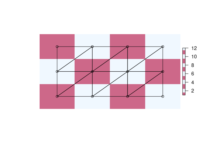
par(op)Quads are trivially converted into triangle form by splitting each in two. Note that this is different again from the centre-based triangle interpretation.
tri2 <- qm
tri2$it <- triangulate_quads(tri2$ib)
tri2$ib <- NULL
tri2$primtivetype <- "triangle"

op <- par(xpd = NA)
plot(extent(r) + 0.5, type = "n", axes = FALSE, xlab = "", ylab = "")
plot(r, col = rep(c("palevioletred3", "aliceblue"), 6), add = TRUE)


points(t(tri2$vb[1:2, ]))
polygon(t(tri2$vb[1:2, head(as.vector(rbind(tri2$it, NA)), -1)]), lwd = 2, lty = 2)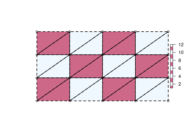
The in-built etopo data set is used to create a plot in
a local map projection. Here each cell is drawn by reprojecting it
directly and individually into this new coordinate system.
library(quadmesh)
library(raster)
## VicGrid
prj <- "+proj=lcc +lat_1=-36 +lat_2=-38 +lat_0=-37 +lon_0=145 +x_0=2500000 +y_0=2500000 +ellps=GRS80 +towgs84=0,0,0,0,0,0,0 +units=m +no_defs"
er <- crop(etopo, extent(110, 160, -50, -20))
system.time(mesh_plot(er, crs = prj))
#>    user  system elapsed
#>   0.147   0.016   0.163

## This is faster to plot and uses much less data that converting explicitly to polygons.

library(sf)
#> Linking to GEOS 3.10.2, GDAL 3.4.3, PROJ 8.2.0; sf_use_s2() is TRUE
p <- st_transform(spex::polygonize(er), prj)
#> old-style crs object detected; please recreate object with a recent sf::st_crs()
plot(st_geometry(p), add = TRUE)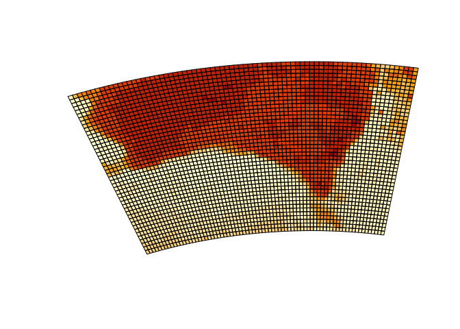
system.time(plot(p, border = NA))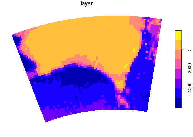
#>    user  system elapsed
#>   0.640   0.022   0.662
pryr::object_size(er)
#> 37.72 kB
pryr::object_size(p)
#> 1.68 MB
pryr::object_size(quadmesh(er))
#> 169.19 kB
The data size and timing benefits are more substantial for larger data sets.
We get exactly what we asked for from mesh_plot, without
the complete remodelling of the data required by grid resampling.
pol <- "+proj=stere +lat_0=-90 +lon_0=147 +datum=WGS84"
mesh_plot(etopo, crs = pol)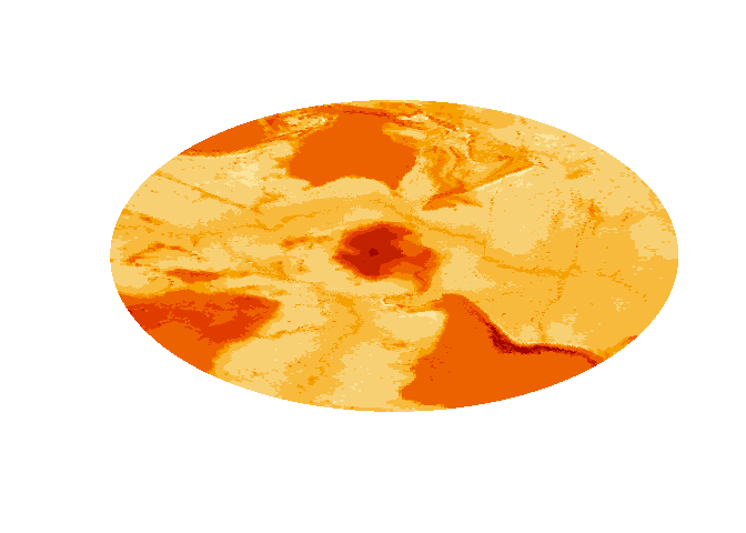
plot(projectRaster(etopo, crs = pol), col = viridis::viridis(64))
#> Warning in wkt(projfrom): CRS object has no comment
#> Warning in wkt(pfrom): CRS object has no comment
#> Warning in rgdal::rawTransform(projfrom, projto, nrow(xy), xy[, 1], xy[, : Using
#> PROJ not WKT2 strings
#> Warning in rgdal::rawTransform(fromcrs, crs, nrow(xy), xy[, 1], xy[, 2]): Using
#> PROJ not WKT2 strings
#> Warning in rgdal::rawTransform(projto_int, projfrom, nrow(xy), xy[, 1], : Using
#> PROJ not WKT2 strings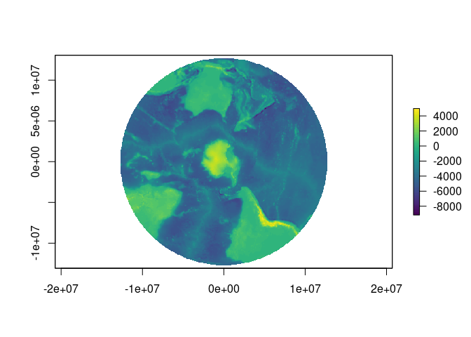
The quadmesh and triangmesh types are
extensions of the rgl class mesh3d, and so are
readily used by that package’s high level functions such as
shade3d() and addNormals().
class(qm)
#> [1] "quadmesh" "mesh3d"   "shape3d"
class(tri)
#> [1] "triangmesh" "mesh3d" "shape3d"The spex package has functions polygonize()
and qm_rasterToPolygons_sp() which provide very fast
conversion of raster grids to a polygon layer with 5 explicit
coordinates for every cell. (stars and sf now
provide an even faster version by using GDAL).
rr <- disaggregate(r, fact = 20)
system.time(spex::polygonize(rr))
#>    user  system elapsed
#>   0.116   0.000   0.116
system.time(raster::rasterToPolygons(rr))
#>    user  system elapsed
#>   1.029   0.000   1.031

## stars has now improved on spex by calling out to GDAL to do the work
system.time(sf::st_as_sf(stars::st_as_stars(rr), merge = FALSE, as_points = FALSE))
#>    user  system elapsed
#> 0.153 0.003 0.156Using a triangulation version of a raster grid we can build an index of weightings for a new of of arbitrary coordinates to estimate the implicit value at each point as if there were continuous interpolation across each primitive.
WIP - see bary_index() function.
Have feedback/ideas? Please let me know via issues.
Many aspects of this package have developed in conjunction with the angstroms package for dealing with ROMS model output.
Please note that this project is released with a Contributor Code of Conduct. By participating in this project you agree to abide by its terms.