{shapviz}

Overview

{shapviz} provides typical SHAP plots:

• sv_importance(): Importance plots (bar plots and/or beeswarm plots).
• sv_dependence() and sv_dependence2D(): Dependence plots to study feature effects and interactions.
• sv_interaction(): Interaction plots.
• sv_waterfall(): Waterfall plots to study single predictions.
• sv_force(): Force plots as alternative to waterfall plots.

SHAP and feature values are stored in a “shapviz” object that is built from:

1. Models that know how to calculate SHAP values: XGBoost, LightGBM, h2o, or
2. SHAP crunchers like {fastshap}, {kernelshap}, {treeshap}, {fastr}, {DALEX}, or simply from a
3. SHAP matrix and its corresponding feature values.

Installation

# From CRAN
install.packages("shapviz")

# Or the newest version from GitHub:
# install.packages("devtools")
devtools::install_github("ModelOriented/shapviz")

Usage

Shiny diamonds… let’s use XGBoost to model their prices by the four “C” variables:

library(shapviz)
library(ggplot2)
library(xgboost)

set.seed(1)

# Build model
x <- c("carat", "cut", "color", "clarity")
dtrain <- xgb.DMatrix(data.matrix(diamonds[x]), label = diamonds$price)
fit <- xgb.train(params = list(learning_rate = 0.1), data = dtrain, nrounds = 65)

# SHAP analysis: X can even contain factors
dia_2000 <- diamonds[sample(nrow(diamonds), 2000), x]
shp <- shapviz(fit, X_pred = data.matrix(dia_2000), X = dia_2000)

sv_importance(shp, show_numbers = TRUE)
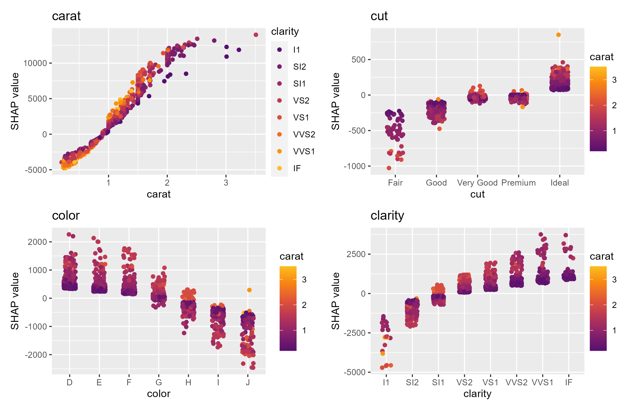
sv_dependence(shp, v = x)

Decompositions of individual predictions can be visualized as waterfall or force plot:

sv_waterfall(shp, row_id = 1)
sv_force(shp, row_id = 1)

More to Discover

Check-out the vignettes for topics like:

• How to work with other SHAP packages like {fastshap}, {kernelshap} or {treeshap}?
• SHAP interactions.
• Multiple models, multi-output models, and subgroup analyses.
• Plotting geographic effects.

References

[1] Scott M. Lundberg and Su-In Lee. A Unified Approach to Interpreting Model Predictions. Advances in Neural Information Processing Systems 30 (2017).