![]()
![]()
![]()
A scalable method to estimates joint Species Distribution Models (jSDMs) based on the multivariate probit model through Monte-Carlo approximation of the joint likelihood. The numerical approximation is based on ‘PyTorch’ and ‘reticulate’, and can be calculated on CPUs and GPUs alike.
The method is described in Pichler & Hartig (2021) A new joint species distribution model for faster and more accurate inference of species associations from big community data.
The package includes options to fit various different (j)SDM models:
To get more information, install the package and run
library(sjSDM)
?sjSDM
vignette("sjSDM", package="sjSDM")sjSDM is based on ‘PyTorch’, a ‘python’ library, and thus requires ‘python’ dependencies. The ‘python’ dependencies can be automatically installed by running:
library(sjSDM)
install_sjSDM()
If this didn’t work, please check the troubleshooting guide:
library(sjSDM)
?installation_helpSimulate a community and fit a sjSDM model:
library(sjSDM)
## ── Attaching sjSDM ──────────────────────────────────────────────────── 1.0.4 ──
## ✔ torch <environment>
## ✔ torch_optimizer
## ✔ pyro
## ✔ madgrad
set.seed(42)
community <- simulate_SDM(sites = 100, species = 10, env = 3, se = TRUE)
Env <- community$env_weights
Occ <- community$response
SP <- matrix(rnorm(200, 0, 0.3), 100, 2) # spatial coordinates (no effect on species occurences)

model <- sjSDM(Y = Occ, env = linear(data = Env, formula = ~X1+X2+X3), spatial = linear(data = SP, formula = ~0+X1:X2), se = TRUE, family=binomial("probit"), sampling = 100L)
summary(model)
## Family:  binomial
##
## LogLik:  -508.7274
## Regularization loss:  0
##
## Species-species correlation matrix:
##
##  sp1  1.0000
##  sp2 -0.3650  1.0000
##  sp3 -0.1910 -0.4300  1.0000
##  sp4 -0.1800 -0.3670  0.8280  1.0000
##  sp5  0.6860 -0.3800 -0.1050 -0.0890  1.0000
##  sp6 -0.2860  0.4900  0.1730  0.1960 -0.0970  1.0000
##  sp7  0.5640 -0.1080  0.1310  0.1630  0.5580  0.2810  1.0000
##  sp8  0.2920  0.1920 -0.5070 -0.5220  0.2050 -0.0380  0.1150  1.0000
##  sp9 -0.0670 -0.0540  0.0480  0.0560 -0.3910 -0.3570 -0.2350 -0.1250  1.0000
##  sp10     0.2110  0.4840 -0.7090 -0.6490  0.2550  0.1420  0.1330  0.4510 -0.2690  1.0000
##
##
##
## Spatial:
##            sp1       sp2      sp3       sp4      sp5     sp6      sp7      sp8
## X1:X2 1.807111 -3.891649 3.616006 0.2416204 2.371867 1.23862 3.087861 1.890661
##            sp9     sp10
## X1:X2 1.237618 1.302866
##
##
##
##                  Estimate  Std.Err Z value Pr(>|z|)
## sp1 (Intercept)  -0.05573  0.27360   -0.20  0.83858
## sp1 X1            1.34006  0.56886    2.36  0.01849 *
## sp1 X2           -2.42857  0.51421   -4.72  2.3e-06 ***
## sp1 X3           -0.27071  0.43979   -0.62  0.53819
## sp2 (Intercept)   0.00232  0.27897    0.01  0.99336
## sp2 X1            1.38987  0.59367    2.34  0.01922 *
## sp2 X2            0.36444  0.50596    0.72  0.47135
## sp2 X3            0.68465  0.43890    1.56  0.11878
## sp3 (Intercept)  -0.55909  0.27776   -2.01  0.04413 *
## sp3 X1            1.49674  0.51045    2.93  0.00337 **
## sp3 X2           -0.47064  0.49361   -0.95  0.34036
## sp3 X3           -1.12252  0.49705   -2.26  0.02392 *
## sp4 (Intercept)  -0.09188  0.23848   -0.39  0.70003
## sp4 X1           -1.55543  0.47517   -3.27  0.00106 **
## sp4 X2           -1.91234  0.45110   -4.24  2.2e-05 ***
## sp4 X3           -0.37758  0.40194   -0.94  0.34752
## sp5 (Intercept)  -0.22248  0.26192   -0.85  0.39564
## sp5 X1            0.76319  0.51134    1.49  0.13556
## sp5 X2            0.56888  0.50411    1.13  0.25911
## sp5 X3           -0.73548  0.45295   -1.62  0.10443
## sp6 (Intercept)   0.30172  0.26113    1.16  0.24792
## sp6 X1            2.66774  0.53908    4.95  7.5e-07 ***
## sp6 X2           -1.09261  0.49401   -2.21  0.02699 *
## sp6 X3            0.19688  0.42018    0.47  0.63938
## sp7 (Intercept)  -0.02088  0.23800   -0.09  0.93009
## sp7 X1           -0.30568  0.47481   -0.64  0.51970
## sp7 X2            0.32681  0.43209    0.76  0.44945
## sp7 X3           -1.51884  0.40833   -3.72  0.00020 ***
## sp8 (Intercept)   0.16312  0.16370    1.00  0.31905
## sp8 X1            0.34875  0.31925    1.09  0.27466
## sp8 X2            0.31206  0.30730    1.02  0.30988
## sp8 X3           -1.20898  0.28881   -4.19  2.8e-05 ***
## sp9 (Intercept)   0.02942  0.19061    0.15  0.87733
## sp9 X1            1.39647  0.37376    3.74  0.00019 ***
## sp9 X2           -1.09693  0.36395   -3.01  0.00258 **
## sp9 X3            0.76818  0.31463    2.44  0.01463 *
## sp10 (Intercept) -0.10078  0.20713   -0.49  0.62656
## sp10 X1          -0.51072  0.37896   -1.35  0.17776
## sp10 X2          -1.23867  0.37494   -3.30  0.00095 ***
## sp10 X3          -0.55472  0.35597   -1.56  0.11916
## ---
## Signif. codes:  0 '***' 0.001 '**' 0.01 '*' 0.05 '.' 0.1 ' ' 1
plot(model)
## Family:  binomial
##
## LogLik:  -508.7274
## Regularization loss:  0
##
## Species-species correlation matrix:
##
##  sp1  1.0000
##  sp2 -0.3650  1.0000
##  sp3 -0.1910 -0.4300  1.0000
##  sp4 -0.1800 -0.3670  0.8280  1.0000
##  sp5  0.6860 -0.3800 -0.1050 -0.0890  1.0000
##  sp6 -0.2860  0.4900  0.1730  0.1960 -0.0970  1.0000
##  sp7  0.5640 -0.1080  0.1310  0.1630  0.5580  0.2810  1.0000
##  sp8  0.2920  0.1920 -0.5070 -0.5220  0.2050 -0.0380  0.1150  1.0000
##  sp9 -0.0670 -0.0540  0.0480  0.0560 -0.3910 -0.3570 -0.2350 -0.1250  1.0000
##  sp10     0.2110  0.4840 -0.7090 -0.6490  0.2550  0.1420  0.1330  0.4510 -0.2690  1.0000
##
##
##
## Spatial:
##            sp1       sp2      sp3       sp4      sp5     sp6      sp7      sp8
## X1:X2 1.807111 -3.891649 3.616006 0.2416204 2.371867 1.23862 3.087861 1.890661
##            sp9     sp10
## X1:X2 1.237618 1.302866
##
##
##
##                  Estimate  Std.Err Z value Pr(>|z|)
## sp1 (Intercept)  -0.05573  0.27360   -0.20  0.83858
## sp1 X1            1.34006  0.56886    2.36  0.01849 *
## sp1 X2           -2.42857  0.51421   -4.72  2.3e-06 ***
## sp1 X3           -0.27071  0.43979   -0.62  0.53819
## sp2 (Intercept)   0.00232  0.27897    0.01  0.99336
## sp2 X1            1.38987  0.59367    2.34  0.01922 *
## sp2 X2            0.36444  0.50596    0.72  0.47135
## sp2 X3            0.68465  0.43890    1.56  0.11878
## sp3 (Intercept)  -0.55909  0.27776   -2.01  0.04413 *
## sp3 X1            1.49674  0.51045    2.93  0.00337 **
## sp3 X2           -0.47064  0.49361   -0.95  0.34036
## sp3 X3           -1.12252  0.49705   -2.26  0.02392 *
## sp4 (Intercept)  -0.09188  0.23848   -0.39  0.70003
## sp4 X1           -1.55543  0.47517   -3.27  0.00106 **
## sp4 X2           -1.91234  0.45110   -4.24  2.2e-05 ***
## sp4 X3           -0.37758  0.40194   -0.94  0.34752
## sp5 (Intercept)  -0.22248  0.26192   -0.85  0.39564
## sp5 X1            0.76319  0.51134    1.49  0.13556
## sp5 X2            0.56888  0.50411    1.13  0.25911
## sp5 X3           -0.73548  0.45295   -1.62  0.10443
## sp6 (Intercept)   0.30172  0.26113    1.16  0.24792
## sp6 X1            2.66774  0.53908    4.95  7.5e-07 ***
## sp6 X2           -1.09261  0.49401   -2.21  0.02699 *
## sp6 X3            0.19688  0.42018    0.47  0.63938
## sp7 (Intercept)  -0.02088  0.23800   -0.09  0.93009
## sp7 X1           -0.30568  0.47481   -0.64  0.51970
## sp7 X2            0.32681  0.43209    0.76  0.44945
## sp7 X3           -1.51884  0.40833   -3.72  0.00020 ***
## sp8 (Intercept)   0.16312  0.16370    1.00  0.31905
## sp8 X1            0.34875  0.31925    1.09  0.27466
## sp8 X2            0.31206  0.30730    1.02  0.30988
## sp8 X3           -1.20898  0.28881   -4.19  2.8e-05 ***
## sp9 (Intercept)   0.02942  0.19061    0.15  0.87733
## sp9 X1            1.39647  0.37376    3.74  0.00019 ***
## sp9 X2           -1.09693  0.36395   -3.01  0.00258 **
## sp9 X3            0.76818  0.31463    2.44  0.01463 *
## sp10 (Intercept) -0.10078  0.20713   -0.49  0.62656
## sp10 X1          -0.51072  0.37896   -1.35  0.17776
## sp10 X2          -1.23867  0.37494   -3.30  0.00095 ***
## sp10 X3          -0.55472  0.35597   -1.56  0.11916
## ---
## Signif. codes:  0 '***' 0.001 '**' 0.01 '*' 0.05 '.' 0.1 ' ' 1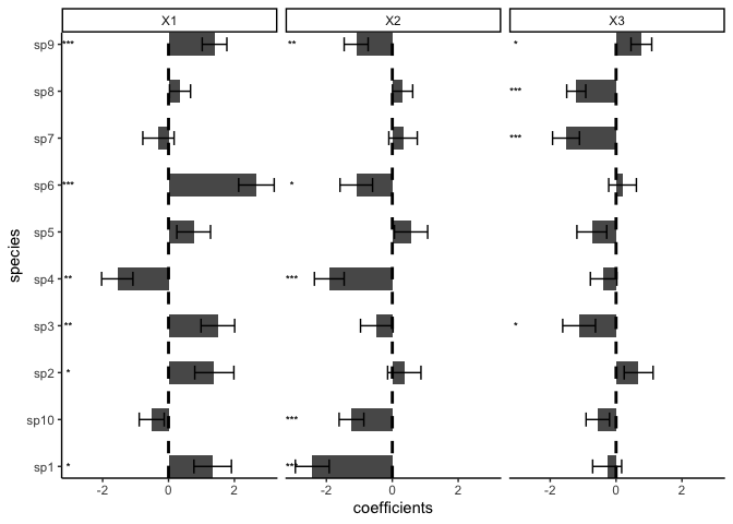
We support other distributions:
Count data with Poisson:
model <- sjSDM(Y = Occ, env = linear(data = Env, formula = ~X1+X2+X3), spatial = linear(data = SP, formula = ~0+X1:X2), se = TRUE, family=poisson("log"))Count data with negative Binomial (which is still experimental, if you run into errors/problems, please let us know):
model <- sjSDM(Y = Occ, env = linear(data = Env, formula = ~X1+X2+X3), spatial = linear(data = SP, formula = ~0+X1:X2), se = TRUE, family="nbinom")Gaussian (normal):
model <- sjSDM(Y = Occ, env = linear(data = Env, formula = ~X1+X2+X3), spatial = linear(data = SP, formula = ~0+X1:X2), se = TRUE, family=gaussian("identity"))ANOVA can be used to partition the three components (abiotic, biotic, and spatial):
an = anova(model)
print(an)
## Analysis of Deviance Table
##
## Terms added sequentially:
##
##           Deviance Residual deviance R2 Nagelkerke R2 McFadden
## Abiotic  157.92268        1177.37216       0.79387      0.1139
## Biotic   175.40897        1159.88588       0.82694      0.1265
## Spatial   16.28744        1319.00741       0.15030      0.0117
## Full     387.13884         948.15601       0.97917      0.2793
plot(an)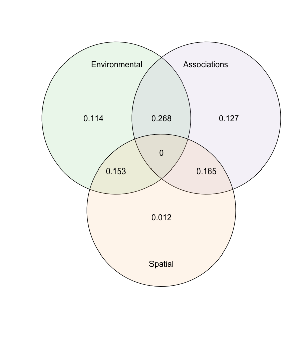
The anova shows the relative changes in the R2 of the groups and their intersections.
Following Leibold et al., 2022 we can calculate and visualize the internal metacommunity structure (=partitioning of the three components for species and sites). The internal structure is already calculated by the ANOVA and we can visualize it with the plot method:
results = plotInternalStructure(an) # or plot(an, internal = TRUE)
## Registered S3 methods overwritten by 'ggtern':
##   method           from
##   grid.draw.ggplot ggplot2
##   plot.ggplot      ggplot2
##   print.ggplot     ggplot2
The plot function returns the results for the internal metacommunity structure:
print(results$data$Species)
##           env         spa     codist         r2
## 1  0.18030741 0.000000000 0.16283743 0.03411591
## 2  0.08715478 0.019089232 0.18394478 0.02901888
## 3  0.11717770 0.013074584 0.20191543 0.03321677
## 4  0.16619488 0.003832403 0.16366855 0.03336958
## 5  0.08432392 0.000000000 0.16981670 0.02522153
## 6  0.18586884 0.000000000 0.11975589 0.03054916
## 7  0.11465238 0.016740799 0.13184580 0.02632390
## 8  0.13783609 0.008329915 0.05558837 0.02017544
## 9  0.16799688 0.014057668 0.04716048 0.02292150
## 10 0.09935810 0.007978024 0.13615356 0.02434897Change linear part of model to a deep neural network:
DNN <- sjSDM(Y = Occ, env = DNN(data = Env, formula = ~.), spatial = linear(data = SP, formula = ~0+X1:X2), se = TRUE, family=binomial("probit"), sampling = 100L)
summary(DNN)
## Family:  binomial
##
## LogLik:  -466.828
## Regularization loss:  0
##
## Species-species correlation matrix:
##
##  sp1  1.0000
##  sp2 -0.4510  1.0000
##  sp3 -0.1620 -0.3370  1.0000
##  sp4 -0.0730 -0.4010  0.8670  1.0000
##  sp5  0.6450 -0.3200 -0.1800 -0.1180  1.0000
##  sp6 -0.3620  0.4120  0.3070  0.1980 -0.0680  1.0000
##  sp7  0.5680 -0.0980  0.1680  0.2080  0.5430  0.2750  1.0000
##  sp8  0.2310  0.1720 -0.5000 -0.5500  0.1380 -0.0170  0.0480  1.0000
##  sp9 -0.0190  0.0530  0.0130  0.0650 -0.4540 -0.4090 -0.2020 -0.0820  1.0000
##  sp10     0.1290  0.4600 -0.7080 -0.7200  0.3200  0.0790  0.1160  0.4290 -0.2620  1.0000
##
##
##
## Spatial:
##            sp1       sp2      sp3       sp4      sp5      sp6      sp7      sp8
## X1:X2 1.763654 -3.796902 3.750247 0.6460114 3.022765 1.352927 3.291612 2.691203
##            sp9     sp10
## X1:X2 1.119004 1.262632
##
##
##
## Env architecture:
## ===================================
## Layer_1:  (4, 10)
## Layer_2:  SELU
## Layer_3:  (10, 10)
## Layer_4:  SELU
## Layer_5:  (10, 10)
## Layer_6:  SELU
## Layer_7:  (10, 10)
## ===================================
## Weights :     340