This package makes it easy to explore trends in Twitter data using the Storywrangler application programming interface (API). Data is returned in a tidy tibble to make it easy to work with and visualize.
For more details about Storywrangler, please see:
You can install the developer version, which has the latest bugfixes and features, with:
devtools::install_github("chris31415926535/storywranglr")You can install the released version of storywranglr from CRAN with:
install.packages("storywranglr")Let’s use storywranglr::ngrams() to chart the popularity
of the 2-gram “black friday” over time. Not surprisingly, it looks like
there’s an annual peak around Black Friday.
library(storywranglr)
library(tidyverse)

result <- storywranglr::ngrams("black friday")

result %>%
  ggplot(aes(x=date, y=rank)) +
  geom_point() +
  theme_minimal() +
  scale_y_continuous(trans = "reverse") +
  labs(title = "Twitter rank popularity of 2-gram 'black friday'",
       subtitle = "Data from Storywrangler ngrams API",
       x = "Date",
       y = "Rank")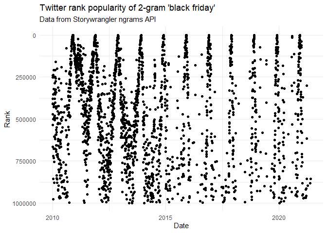
Now using storywrangler::zipf(), let’s find the 10 top
2-grams from January 6, 2021. “the Capitol” made the top 10, and if we
got a longer list we could expect to see other thematically related
terms.
result <- zipf("2021-01-06", max = 10, ngrams = 2)

knitr::kable(result)| ngram | count | count_no_rt | rank | rank_no_rt | freq | freq_no_rt | odds | date |
|---|---|---|---|---|---|---|---|---|
| of the | 1327429 | 236481 | 2 | 3 | 0.0026367 | 0.0018889 | 379.2560 | 2021-01-06 |
| in the | 1116763 | 236362 | 3 | 4 | 0.0022183 | 0.0018880 | 450.7987 | 2021-01-06 |
| the Capitol | 813958 | 43687 | 5 | 75 | 0.0016168 | 0.0003490 | 618.5029 | 2021-01-06 |
| This is | 684264 | 140136 | 6 | 8 | 0.0013592 | 0.0011193 | 735.7326 | 2021-01-06 |
| to the | 610598 | 122263 | 8 | 13 | 0.0012129 | 0.0009766 | 824.4956 | 2021-01-06 |
| on the | 601955 | 114038 | 9 | 15 | 0.0011957 | 0.0009109 | 836.3339 | 2021-01-06 |
| to be | 588970 | 169747 | 10 | 5 | 0.0011699 | 0.0013559 | 854.7725 | 2021-01-06 |