![]()
![]()
The goal of tidysmd is to easily create tidy data frames of SMDs. tidysmd wraps the smd package to easily calculate SMDs across many variables and using several weights in order to easily compare different adjustment strategies.
You can install the most recent version of tidysmd from CRAN with:
install.packages("tidysmd")Alternatively, you can install the development version of tidysmd from GitHub with:
# install.packages("devtools")
devtools::install_github("malcolmbarrett/tidysmd")tidy_smd() supports both unweighted SMDs and weighted
SMDs.
library(tidysmd)
tidy_smd(nhefs_weights, c(age, education, race), .group = qsmk)
#> # A tibble: 3 × 4
#>   variable  method   qsmk     smd
#>   <chr>     <chr>    <chr>  <dbl>
#> 1 age       observed 1     -0.282
#> 2 education observed 1      0.196
#> 3 race      observed 1      0.177
nhefs_weights contains several types of propensity score
weights for which we can calculate SMDs. Unweighted SMDs are also
included by default.
tidy_smd(
  nhefs_weights,
  c(age, race, education),
  .group = qsmk,
  .wts = c(w_ate, w_att, w_atm)
)
#> # A tibble: 12 × 4
#>    variable  method   qsmk       smd
#>    <chr>     <chr>    <chr>    <dbl>
#>  1 age       observed 1     -0.282
#>  2 race      observed 1      0.177
#>  3 education observed 1      0.196
#>  4 age       w_ate    1     -0.00585
#>  5 race      w_ate    1      0.00664
#>  6 education w_ate    1      0.0347
#>  7 age       w_att    1     -0.0120
#>  8 race      w_att    1      0.00365
#>  9 education w_att    1      0.0267
#> 10 age       w_atm    1     -0.00184
#> 11 race      w_atm    1      0.00113
#> 12 education w_atm    1      0.00934
Having SMDs in a tidy format makes it easy to work with the
estimates, for instance in creating Love plots. tidysmd includes
geom_love() to make this a bit easier:
library(ggplot2)
plot_df <- tidy_smd(
  nhefs_weights,
  race:active,
  .group = qsmk,
  .wts = starts_with("w_")
)

ggplot(
  plot_df,
  aes(
    x = abs(smd),
    y = variable,
    group = method,
    color = method,
    fill = method
  )
) +
  geom_love()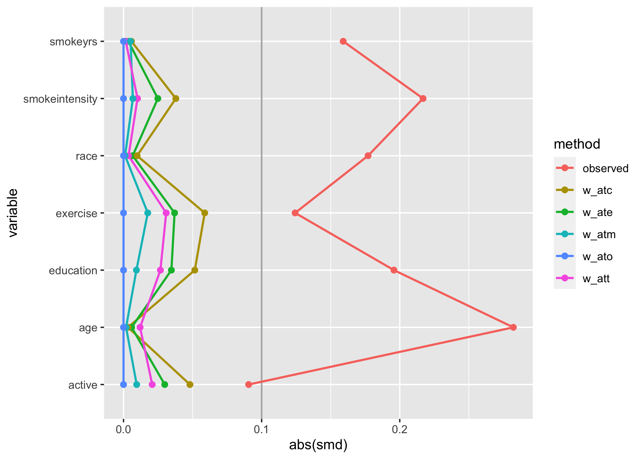
You can also use the quick-plotting function
love_plot(), if you prefer:
love_plot(plot_df) +
  theme_minimal(14) +
  ylab(NULL)
tidysmd also has support for working with matched datasets. Consider these two objects from the MatchIt documentation:
library(MatchIt)
# Default: 1:1 NN PS matching w/o replacement
m.out1 <- matchit(treat ~ age + educ + race + nodegree +
                   married + re74 + re75, data = lalonde)

# 1:1 NN Mahalanobis distance matching w/ replacement and
# exact matching on married and race
m.out2 <- matchit(treat ~ age + educ + race + nodegree +
                   married + re74 + re75, data = lalonde,
                   distance = "mahalanobis", replace = TRUE,
                  exact = ~ married + race)
One option is to just look at the matched dataset with tidysmd:
matched_data <- get_matches(m.out1)

match_smd <- tidy_smd(
  matched_data,
  c(age, educ, race, nodegree, married, re74, re75),
  .group = treat
)

love_plot(match_smd)
The downside here is that you can’t compare multiple matching
strategies to the observed dataset; the label on the plot is also wrong.
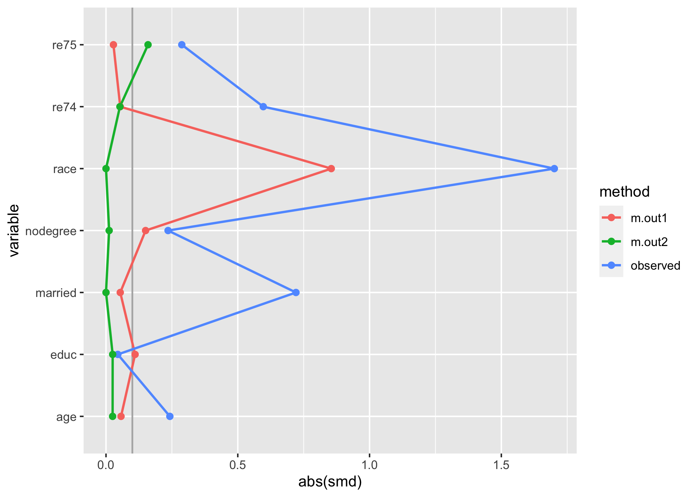
tidysmd comes with a helper function, bind_matches(), that
creates a dataset more appropriate for this task:
matches <- bind_matches(lalonde, m.out1, m.out2)
head(matches)
#>      treat age educ   race married nodegree re74 re75       re78 m.out1 m.out2
#> NSW1     1  37   11  black       1        1    0    0  9930.0460      1      1
#> NSW2     1  22    9 hispan       0        1    0    0  3595.8940      1      1
#> NSW3     1  30   12  black       0        0    0    0 24909.4500      1      1
#> NSW4     1  27   11  black       0        1    0    0  7506.1460      1      1
#> NSW5     1  33    8  black       0        1    0    0   289.7899      1      1
#> NSW6     1  22    9  black       0        1    0    0  4056.4940      1      1
matches includes an binary variable for each
matchit object which indicates if the row was included in
the match or not. Since downweighting to 0 is equivalent to filtering
the datasets to the matches, we can more easily compare multiple matched
datasets with .wts:
many_matched_smds <- tidy_smd(
  matches,
  c(age, educ, race, nodegree, married, re74, re75),
  .group = treat,
  .wts = c(m.out1, m.out2)
)

love_plot(many_matched_smds)