![]()
![]()
![]()
The goal of traipse is to provide shared tools for tracking data, for
common metrics of distance, direction, and speed. The package includes
the following functions which are always assumed to operate on input
locations in longitude latitude, and input date-times in R’s
POSIXt class.
track_distance() for distance in metrestrack_angle() for internal angle in degreestrack_turn() for relative turn angletrack_bearing() for absolute bearingtrack_time() for duration in secondstrack_speed() for speed in metres per secondtrack_distance_to() for distance to locationtrack_bearing_to() for bearing to locationtrack_intermediate() for interpolating locationstrack_query() also for interpolation, by finding
locations within a given track arbitrarily (in-development)track_grid for identifying locations in grid cellsDistances are always returned in metres, directions
and angles are always returned in degrees. Absolute
bearing is relative to North (0), and proceeds clockwise positive and
anti-clockwise negative
N = 0, E = 90, S = +/-180, W = -90.
Time is always returned in seconds, and speed in metres per second.
Traipse works directly on longitude and latitude vectors as it is intended for use within other tools that work directly with data.
There is no capacity for providing nested data structures because this is trivially done by using tidyverse code like
data %>% group_by(id) %>% mutate(distance = track_distance(lon, lat)) %>% ungroup()or by arranging use of the functions in various ways. Track metric
values are inherently window-like
and in traipse padding value/s of NA are used to return an
element for every input location.
You can install traipse from CRAN with:
install.packages("traipse")You can install the development version from GitHub with:
# install.packages("devtools")
devtools::install_github("Trackage/traipse")This is a basic example which shows you how to calculate ellipsoidal distance and turning angle for a data set of tracks.
First, calculate without any groupings - we definitely don’t want
this for real work as there are three separate tracks within our data
set identified by id. (No ordering is applied other than
the order the rows occur).
library(traipse)

library(dplyr)
## there's no grouping here - we haven't gotten our data organized yet
trips0 %>% mutate(distance = track_distance(x, y), angle = track_angle(x, y))
#> # A tibble: 1,500 × 6
#>        x     y date                id    distance  angle
#>    <dbl> <dbl> <dttm>              <chr>    <dbl>  <dbl>
#>  1  115. -42.4 2001-01-01 15:39:50 1          NA   NA
#>  2  116. -41.4 2001-01-01 18:16:52 1      129435. 120.
#>  3  116. -41.1 2001-01-01 21:03:38 1       34632.   4.43
#>  4  117. -42.1 2001-01-01 22:09:41 1      120575.  13.1
#>  5  116. -41.9 2001-01-01 23:33:54 1       30560.  72.4
#>  6  118. -42.0 2001-01-02 01:25:12 1       97593.  25.6
#>  7  117. -41.7 2001-01-02 06:45:40 1       57005.  89.5
#>  8  118. -40.9 2001-01-02 10:01:26 1      108811. 159.
#>  9  118. -39.7 2001-01-02 13:49:59 1      130588.  23.8
#> 10  118. -40.5 2001-01-02 16:24:46 1       86066.  64.3
#> # … with 1,490 more rows
Now run a set of available metrics, but do it with respect to the
grouping variable id.
metric <- trips0 %>% group_by(id) %>% mutate(distance = track_distance(x, y),
                                             angle = track_angle(x, y),
                                             turn = track_turn(x, y),
                                             bearing = track_bearing(x, y),
                                             duration = track_time(date),
                                             speed = track_speed(x, y, date),
                                             distance_to = track_distance_to(x, y, 147, -42),
                                             bearing_to = track_bearing_to(x, y, 100, -42))
metric
#> # A tibble: 1,500 × 12
#> # Groups:   id [3]
#>        x     y date                id    distance  angle   turn bearing duration
#>    <dbl> <dbl> <dttm>              <chr>    <dbl>  <dbl>  <dbl>   <dbl>    <dbl>
#>  1  115. -42.4 2001-01-01 15:39:50 1          NA   NA      NA     34.5        NA
#>  2  116. -41.4 2001-01-01 18:16:52 1      129435. 120.    -61.0  -26.5      9422
#>  3  116. -41.1 2001-01-01 21:03:38 1       34632.   4.43 -175.   158.      10006
#>  4  117. -42.1 2001-01-01 22:09:41 1      120575.  13.1  -167.    -9.20     3963
#>  5  116. -41.9 2001-01-01 23:33:54 1       30560.  72.4   108.    98.5      5053
#>  6  118. -42.0 2001-01-02 01:25:12 1       97593.  25.6  -155.   -56.7      6678
#>  7  117. -41.7 2001-01-02 06:45:40 1       57005.  89.5    90.9   34.1     19228
#>  8  118. -40.9 2001-01-02 10:01:26 1      108811. 159.    -21.2   12.9     11746
#>  9  118. -39.7 2001-01-02 13:49:59 1      130588.  23.8   156.   169.      13713
#> 10  118. -40.5 2001-01-02 16:24:46 1       86066.  64.3  -116.    53.1      9287
#> # … with 1,490 more rows, and 3 more variables: speed <dbl>, distance_to <dbl>,
#> #   bearing_to <dbl>

metric %>%
  ggplot(aes(x, y, cex= 1/angle)) +
  geom_point() +
  geom_path(col = rgb(0.2, 0.2, 0.2, 0.2))
#> Warning: Removed 6 rows containing missing values (geom_point).
#> Warning: Removed 2 row(s) containing missing values (geom_path).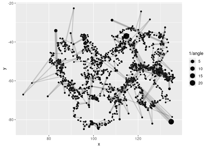
metric %>%
  ggplot(aes(x, y, colour = distance_to)) +
  geom_point() + geom_label(data = data.frame(x = 147, y = -42, distance_to = 0),
                            label = "home")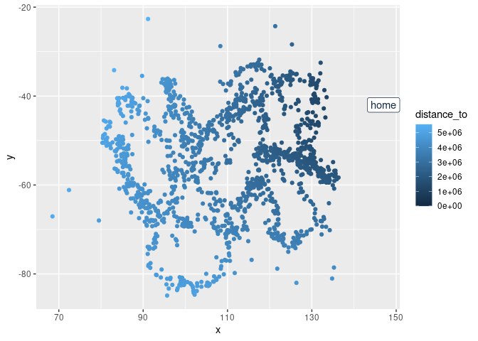
metric %>%
  ggplot(aes(x, y, colour = bearing_to)) +
  geom_point() + geom_label(data = data.frame(x = 100, y = -42, bearing_to = 0),
                            label = "home")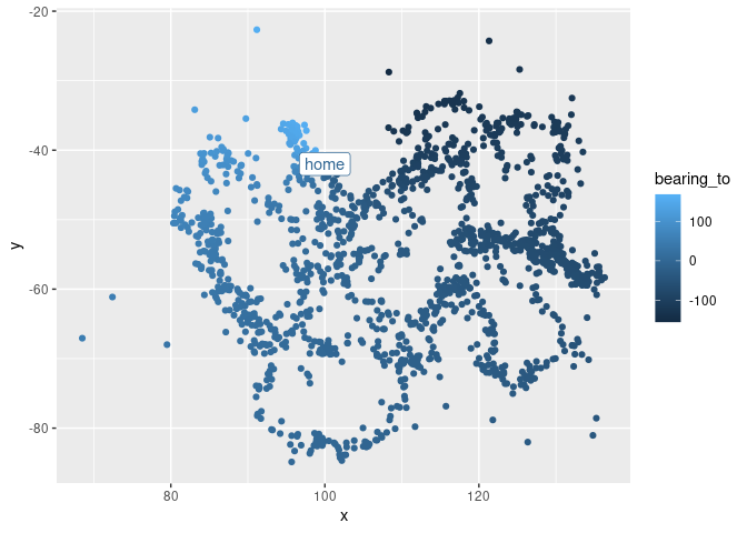
Using the bearing and distance now reproduce the track as destination point segments.
plot(metric[1:10, c("x", "y")], type = "b", lwd = 10, col = "grey")
dest <- geosphere::destPoint(metric[1:10, c("x", "y")],
                             b = metric$bearing[1:10],
                            d = metric$distance[2:11])
arrows(metric$x[1:10], metric$y[1:10], dest[1:10,1], dest[1:10,2], col = "firebrick", lwd = 2)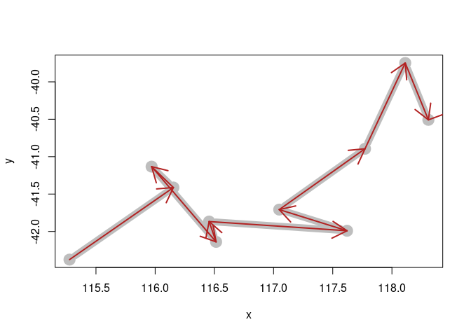
The function track_intermediate() requires extra work as
it inherently returns multiple variables (lon, lat, date-time). The
output is a list-column of data frames, and if used within
mutate(inter = track_intermediate(lon, lat, date)) then it
will be stored along side the rows of the input data.
To use this we must unnest the data and treat the new columns as the output.
See this example.
if (requireNamespace("tidyr") && requireNamespace("dplyr")) {
tr1 <- trips0[seq(1, nrow(trips0), by = 30), ]
dd <- tr1 %>% group_by(id) %>%
mutate(inter = track_intermediate(x, y, date = date, distance = 150000)) %>%
tidyr::unnest()
plot(dd$int_date, dd$int_y, pch = ".", cex = 2, main = "equidistant in space")
abline(v = tr1$date)
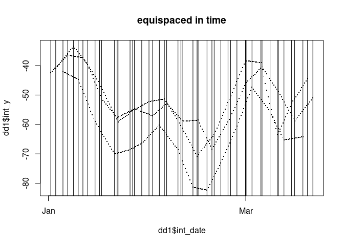
dd1 <- tr1 %>% group_by(id) %>%
mutate(inter = track_intermediate(x, y, date = date, duration = 3600 * 12)) %>%
tidyr::unnest()
plot(dd1$int_date, dd1$int_y, pch = ".", cex = 2, main = "equispaced in time")
abline(v = tr1$date)
}
#> Warning: `cols` is now required when using unnest().
#> Please use `cols = c(inter)`
#> `cols` is now required when using unnest().
#> Please use `cols = c(inter)`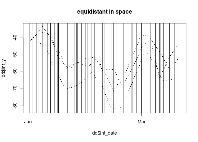
Query.
track_query(trips0$x[1:10], trips0$y[1:10], query = c(4.5, 5.5, 6.5))
#> Warning in track_query(trips0$x[1:10], trips0$y[1:10], query = c(4.5, 5.5, :
#> date is null, so assuming linear relative movement in time
#> # A tibble: 3 × 3
#>       x     y  date
#>   <dbl> <dbl> <dbl>
#> 1  116. -42.0   4.5
#> 2  117. -41.9   5.5
#> 3  117. -41.8   6.5
track_query(trips0$x[1:10], trips0$y[1:10], trips0$date[1:10], query = trips0$date[1:10] + 10)
#> # A tibble: 10 × 3
#>        x     y date
#>    <dbl> <dbl> <dttm>
#>  1  115. -42.4 2001-01-01 15:40:00
#>  2  116. -41.4 2001-01-01 18:17:02
#>  3  116. -41.1 2001-01-01 21:03:48
#>  4  117. -42.1 2001-01-01 22:09:51
#>  5  116. -41.9 2001-01-01 23:34:04
#>  6  118. -42.0 2001-01-02 01:25:22
#>  7  117. -41.7 2001-01-02 06:45:50
#>  8  118. -40.9 2001-01-02 10:01:36
#>  9  118. -39.7 2001-01-02 13:50:09
#> 10   NA   NA   2001-01-02 16:24:56
s <- seq(min(trips0$date), max(trips0$date), by = "1 hour")
trips0 %>% group_by(id) %>% group_modify(~track_query(.x$x, .x$y, .x$date, query = s))
#> # A tibble: 5,751 × 4
#> # Groups:   id [3]
#>    id        x     y date
#>    <chr> <dbl> <dbl> <dttm>
#>  1 1       NA   NA   2001-01-01 15:24:58
#>  2 1      116. -42.1 2001-01-01 16:24:58
#>  3 1      116. -41.7 2001-01-01 17:24:58
#>  4 1      116. -41.4 2001-01-01 18:24:58
#>  5 1      116. -41.3 2001-01-01 19:24:58
#>  6 1      116. -41.2 2001-01-01 20:24:58
#>  7 1      116. -41.5 2001-01-01 21:24:58
#>  8 1      117. -42.1 2001-01-01 22:24:58
#>  9 1      116. -41.9 2001-01-01 23:24:58
#> 10 1      117. -41.9 2001-01-02 00:24:58
#> # … with 5,741 more rowsNote above that we provided a grouping ID for when we have separate trips within the same data set. There’s nothing to stop from calculating distances when the arrangement of records does not make sense, but this is your responsibility. If missing values are present, or times are out of order, or include zero-length time durations, or movement backward in time there aren’t any checks for that made in the traipse package.
The idea is for developers to be able to use these tools however they like but with an assumed consistent workflow.
We would like to have a simple core package to provide the most
commonly used metrics. We assume geodist and
geosphere as good examples of core packages for the
underlying tool. These both apply the modern geodesic methods of C. F.
F. Karney (2013) Algorithms for
geodesics
Please note that this project is released with a Contributor Code of Conduct. By contributing to this project, you agree to abide by its terms.